Numerical Methods

In this course, we have solved by hand certain types of differential equations (linear equations, separable equations, and exact equations) using analytic techniques. Unfortunately, the vast majority of differential equations of the form ^dy⁄_dt = ƒ(t,y) are not linear, separable, or exact. For this reason, we need to think about other possible ways to analyze first-order initial value problems. The techniques for finding approximate solutions to differential equation problems using estimation and calculation rather than analytic manipulation are collectively called numerical methods. When we use numerical methods, we don't get a nice formula as a solution to our initial value problem. We do, however, get a way to calculate an approximate value for the solution at any point we choose.

Consider the following initial value problem:

(1)	dy⁄dx = x2 - y3 y(0) = 0

The differential equation in (1) is not linear (because of the y³), nor is it separable or exact. Convince yourself of this with a pencil and paper.

We have no symbolic methods for solving this equation. Thus we will need to use the numerical methods mentioned above. One way we can get an idea of what the solutions to this (or any) differential equation look like is with a direction field. We've already seen in Assignment 2 how to use slopefield and drawode to get a picture of our solution.

>> f = @(x,y) x^2 - y^3;
slopefield(f, [-10,10], [-10,10], 30)
hold on
drawode(f, [-10,10], 0, 0)
hold off

When you run these commands, you will get a warning: MATLAB says it is "unable to meet integration tolerances without reducing the step size." In this case, the curve becomes so steep on the left side that the computer cannot accurately compute more points to plot in a reasonable time. What does that suggest to us about this solution curve?

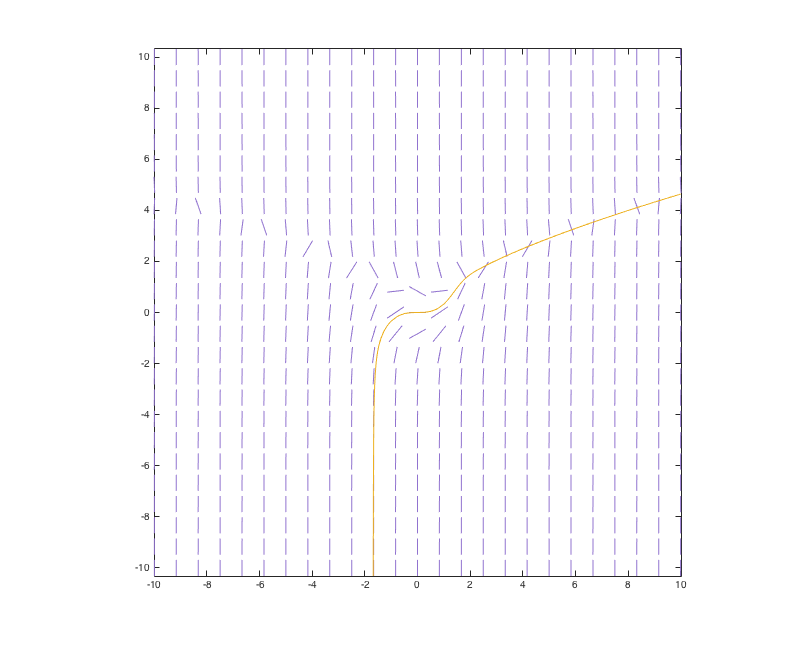
Pictures like these are very informative for understanding the behavior of the solutions to even very complicated differential equations. Unfortunately, such graphical techniques are limited to three dimensions at best. Indeed, most technology problems involve high-dimensional systems of ODEs, so that it is impossible to visualize their solutions. Even with two- or three-dimensional systems, visual techniques might fail us when we want to get very precise information. For example, we might want to find out the value of y in our solution above when x = 10. From the direction field, we can guess that it is somewhere around 4.3. By changing the axes in slopefield, we might be able to zoom in and improve this estimate, but that can be an awkward way to obtain a highly accurate answer.

Thinking about direction fields and their limitations leads us to two questions.

• Q1. What do we do for large systems?
• Q2. How does drawode actually compute solution curves? After all, it is dangerous to run programs without having a solid idea how they work; if you do, eventually you will make a serious mistake.

In this lab we shall try to give you the basic idea behind answers to both Q1 and Q2, although going there from our sketch here is a pretty big leap. (Numerical analysis is, after all, an entire branch of mathematics!) We will explore a couple of numerical methods, beginning with a relatively simple method called Euler's Method. It is the most easily-understood example of a numerical approach to solving differential equations.

Euler's Formula: A Numerical Method

Euler's Method is one of the simplest and oldest numerical methods for approximating solutions to differential equations that cannot be solved with a nice formula. Euler's Method is also called the tangent line method, and in essence it is an algorithmic way of plotting an approximate solution to an initial value problem through the direction field. It can also be used to get an estimated value for that solution at a given value for x. Here is how it works:

To see Euler's Method in use, let's try an example.

Keep this example in mind; we will soon verify these calculations using MATLAB.

Implementing Euler's Formula in MATLAB

We are going to execute Euler's Method in MATLAB using M-Files. It is possible to simply type the necessary commands into the MATLAB window, but this is inefficient. As we saw back in Assignment 1, the advantage to using M-Files instead is that each time we want to run Euler's Method, we can do so with a single command, rather than retyping a long list of commands. In the same way that we defined new functions with M-Files before, we will now define the (more complicated) function Euler. The content of Euler may seem daunting at first, but we will return to explaining how it works after a quick application.

We will need an M-File that runs Euler's Method, so in MATLAB, use the button New or New Script. This will open a new M-file. In this M-File, we will create a function Euler that will take five parameters: h, x0, y0, interval_length, and func. The first four parameters should be numerical values, where h is a number greater than 0. The last parameter func should be a function of two variables, which we will identify as x and y. Using these inputs, Euler will apply Euler's Method to the differential equation ^dy⁄_dx = func on the interval [x0, x0 + interval_length], using a step size of h, going through the point (x0, y0).

When the M-File editor appears, enter (or copy and paste) the following blue text:

1
2
3
4
5
6
7
8
9
10

function [x,y] = Euler(h, x0, y0, interval_length, func)
nsteps = floor(interval_length/h) + 1;
x = zeros(nsteps,1);
y = zeros(nsteps,1);
x(1) = x0;
y(1) = y0;
for i=2:nsteps
    y(i) = y(i-1) + h* func(x(i-1), y(i-1));
    x(i) = x(i-1) + h;
end

Now select the Save button and save the file as Euler.m. (This name will most likely appear in the box for you.) The file should be saved in a directory where MATLAB can access it. If you are working on an ETS machine, you should be able to use your My Documents folder. If you are not working on an ETS machine, make sure you are saving the file into MATLAB's current directory on your machine. (Remember that if you choose to work on non-ETS computers, you do so at your own risk. The TAs cannot provide technical support anywhere outside the designated MATLAB lab.)

We can now use the command Euler from our MATLAB command window. In the previous section above, we went through Euler's Formula for the initial value problem (2) on the interval 0 ≤ x ≤ 2, with h = 0.5. Let's run this again using our new MATLAB command. In the MATLAB command window, type:

This defines our function ^dy⁄_dx = f(x,y) = x² - 1 as a function of two variables, x and y. Now let's run an iteration of Euler's Method:

>> h = 0.5;
[x,y] = Euler(h, 0, 1, 2, f);
[x,y]

The results from running Euler's Method are contained in two arrays, x and y. When we enter the last command [x,y] (note the absence of a semicolon), MATLAB outputs the x and y coordinates of the points computed by Euler's Method. Note that for this example, the output matches what we got at the end of Example 3.2. This is a good sign; Euler can compute the points predicted by Euler's Method without the need to do computations by hand. We can also plot these points graphically by typing:

>> plot(x, y, 'r')
hold on

The 'r' tells MATLAB to draw the graph in red, and as we've seen before, the hold on command will keep the existing graph while you plot more graphs on top of it in the following exercise.

1. Run Euler's Method again, this time for h = 0.2. Plot the results in blue this time. (Use 'b' instead of 'r'.) Look at the arrays x and y side-by-side by typing in
   
   >> [x,y]
   
   Copy the long table of data that you just produced into your Word document. What estimates did the Euler Method come up with for y at x = 1 and x = 2 using this smaller value of h? Now run Euler's Method for h = 0.1 and again for h = 0.01, and plot the results in green ('g') and cyan ('c'), respectively. What are the estimates for y at x = 1 and x = 2 for these values of h? Write these down in your Word document, along with your graph with all four colored curves. (You need not include the data tables for these last two values of h.)
2. The differential equation given in (2) is separable. Calculate the solution to the initial value problem by hand, and use MATLAB (or a calculator) to compute the actual values for y at x = 1 and x = 2. Make sure to include your manual work in your Word document. (You can simply type it.)
3. Does Euler's estimate appear to give better or worse estimates for the solution as h decreases? Give a brief reasoning for why this might be the case. Does Euler's estimate appear to give better or worse estimates for the actual solution as you move farther from the initial point?

Now that we have seen Euler in action, let's return to examining the content of the M-File Euler.m. We have already explained the first line, where we defined the parameters our function takes. To see the meaning behind the third and fourth lines, type:

>> x = zeros(10,1);
y = zeros(10,1);
[x,y]

Thus we can see that the third and fourth lines of our M-File zero out the contents of our arrays x and y before we begin. Now, you'll continue examining our code.

In your Word document, briefly explain what is happening in each remaining line of the M-File Euler.m.

The algorithm we used to implement Euler's Method works when we have a single differential equation. It is worth mentioning, however, that Euler's Method readily generalizes to large systems of differential equations.

Experimenting with Euler's Formula

Let's return to our first example:

We noticed before that there is no way for us to solve this system by any analytic method, but since x² - y³ is a continuous function, we know that a solution exists on some interval around the initial value x = 0. We saw using slopefield and drawode roughly what the solution curve looks like. Now let's use our new numerical method to estimate the solution.

1. Run Euler's Method in MATLAB for the inital value problem (1) on the interval 0 ≤ x ≤ 4. Use different colors to plot the estimates for the following values of h: 1, 0.5, 0.25, and 0.1. Remember to use hold on! Some of the colors you can use with MATLAB's plot command are 'r', 'g', 'b', 'c', 'm', 'y', and 'k'.
   
   Notice that the y-axis is very large. Rescale the y-axis to range from -10 to 10. (Assignment 1 showed us how to do this.) Given the results of the plot, what can you say about the accuracy of the h = 0.1 case? You do not need to include the actual data in the table [x,y] in your writeup, only the plot and your written answer.
2. Enter hold off so that MATLAB will overwrite your previous plot, and this time, run Euler's Method with the h values 1, 0.1, 0.01, and 0.001. Plot the results on one graph using colors of your choice, and rescale so that y ranges from 0 to 2.5. Paste this plot into your writeup.
   
   Did the additional shrinking of h change the results significantly? What does this suggest about the accuracy of your solution for each step size? Comment on the consistency of your plot with the direction field shown at the top of the page, and also describe any inconsistencies between different step sizes.

This example serves as an excellent warning about some of the hazards that may arise when using numerical methods to solve differential equations. Since the answers are by definition not exact, one should be wary of using numerical results without some way to detect inaccuracy.

ODE45

Happily for our sanity, we do not have to go through the steps above to use numerical methods in MATLAB, because MATLAB has a number of numerical methods built in. One of these is ode45, which runs a numerical method of a type collectively known as the Runge-Kutta Methods. These methods are generally more powerful than Euler's Method.

We don't want to go into much detail on the mathematics behind Runge-Kutta, but there is an informative analogy to Taylor expansions. In Euler's Method, we used the tangent line (which is the first order Taylor polynomial) to approximate our solutions. In essence, Runge-Kutta Methods use higher order Taylor polynomial approximations.

Let's try to use the ode45 command now.

Consider the differential equation ^dy⁄_dx = sin(x). We'll first define a function g(x,y) to represent ^dy⁄_dx:

>> g = @(x,y) sin(x)

Now type the following command into MATLAB:

>> [x,y] = ode45(g, [0, 10], 1)

This tells MATLAB to set y, as a function of x, to be the approximation obtained using ode45 to the solution of the ODE we're looking at on the interval [0,10]. The last parameter, the 1, gives the initial condition y(0) = 1. Now that we've done this, we can use the plot command the same way we did before to see a graph of ode45's estimate of the solution.

The differential equation we just looked at is quite easy to solve symbolically. Let's do that.

1. As can be easily verified, the solution to the initial value problem in Example 3.3 is
   
   h(x) = -cos(x) + 2
   
   Now with the solution of the above differential equation, we can compare the results obtained by using ode45 to the actual values. Type the following commands into MATLAB:
   

   >> h = @(x) -cos(x) + 2;
   [x, y, h(x), abs(y - h(x))]

   Include this code and the output in your writeup. The second and third columns give us the estimate that we found using ode45 and the actual function value at each specified value of x. How do the values in the two columns compare? The fourth column gives the absolute value of the difference between the function and our approximation; this is the error of our approximation.
2. Now let us compare the results that ode45 gives us with the results we would get from using Euler's method. Enter the following commands into MATLAB:
   

   >> [x, z] = Euler(0.25, 0, 1, 10, g);
   [y, z, h(x), abs(y - h(x)), abs(z - h(x))]

   Copy the input and output to your Word document. In the first column, we have the results of ode45; in the second, the results of our Euler's Method routine; and in the third, the values at x of the real solution to our differential equation. Columns four and five give the error of ode45 and of Euler's Method, respectively. Which method seems to give more accurate answers in this situation?

We emphasize two features of ode45. First, the algorithm is more powerful than Euler's Method. Second, go back and take a careful look at the parameters we plugged into ode45; there are relatively few of them. Notice that there is no step size parameter, nor is there any other parameter that we may vary to adjust the precision of our calculations. These are picked automatically by the program (a feature of the ode45 implementation, not fundamental to Runge-Kutta Methods). In Exercise 3.4, we were able to test the results of ode45 explicitly because we could solve the differential equation by hand, but in practice, one should remember to search for inaccuracy before using numerical results.

We can now answer one of the questions asked earlier. At the beginning of this lab, we asked how drawode works. As a matter of fact, drawode simply calls ode45 twice, once running forwards in time and once running backwards. So we can think of drawode as using high-degree polynomials to approximate solutions to initial value problems.

Furthermore, Runge-Kutta algorithms generalize from a single ODE to a system of ODEs with very little conceptual difference. In fact, the command ode45 can also be used on systems of differential equations. If you're curious, type help ode45.

Conclusion

The power of computing is best exploited when calculating numerical solutions. In most cases, if a differential equation has a solution, then that solution can be at least closely approximated numerically. One must be a little careful, however. There are many equations that are considered stiff, meaning that some numerical methods for solving them exhibit unstable behavior unless the step size is taken to be very small (as in Exercise 3.3). This is certainly true with Euler's method. The ode45 solver is an all-around tool that does a decent job for many of the equations that come up frequently. In practice, though, one deals with stiff equations by using higher-order numerical methods. This is actually what we just did. Euler's Method is a first-order method (since we use linear approximations), while ode45 is a fourth-order method. MATLAB also offers other solvers, such as ode15s or ode23s. If you're interested, you can type doc and then search there for ODE solvers to learn more about the specific properties of each numerical solver.

In the next lab, we will examine systems of differential equations in more detail. It is important to know that many numerical methods, including both Euler's Method and ode45, can handle systems of differential equations with only minor modification.