The commands NCProcess1 and NCProcess2 were briefly described in §13. In this chapter, we derive a theorem due to Bart, Gohberg, Kaashoek and Van Dooren. The reader can skip the statement of this theorem (§14.1) if he wishes and go directly to the algebraic problem statement (§14.2).
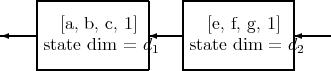
Theorem([BGKvD]) A minimal factorization
of a system [A,B,C, 1] corresponds to projections P1 and P2 satisfying P1 + P2 = 1,
 | (14.1) |
provided the state dimension of the [A,B,C, 1] system is d1 + d2. (which has the geometrical interpretation that A and A - BC have complimentary invariant subspaces).
We begin by giving the algebraic statement of the problem. Suppose that these factors exist. By the Youla-Tissi statespace isomorphism theorem, there is map
 | (14.2) |
which intertwines the original and the product system. Also minimality of the factoring is equivalent to the existence of a two sided inverse (n1T ,n 2T )T to (m 1,m2). These requirements combine to imply that each of the following expressions is zero.
Minimal factors exist if and only if there exist m1, m2, n1, n2, a, b, c, e, f and g such that the following polynomials is zero.
The problem is to solve these equations. That is, we want a constructive theorem which says when and how they can be solved.
We now apply a strategy to see how one might discover this theorem. The formalities of what a strategy is are not important here. This chapter is designed to illustrate NCProcess and allied commands. For a description of the formalities of a strategy see [HS] or for a sketch see Chapter 16.
Before running NCProcess1, we must declare A, B and C to be knowns and the remaining variables to be unknowns. The “**” below denotes matrix multiplication.
In[1]:=Get["NCGB.m"];
In[2]:=SetNonCommuative[A,B,C0,m1,m2,n1,n2]; In[3]:=SetKnowns[A,B,C]; In[4]:=SetUnknowns[m1,m2,n1,n2,a,b,c,e,f,g]; |
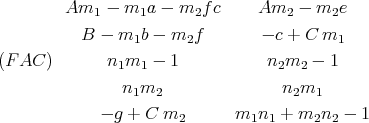
We now set the variable FAC equal to the list of polynomials in §14.2.
In[5]:=FAC = {A**m1 - m1**a - m2**f**c,
A**m2 - m2**e, B - m1**b - m2**f, -c + C0**m1, -g + C0**m2, n1**m1 - 1, n1**m2, n2**m1, n2**m2 - 1, m1**n1 + m2**n2 - 1}; |
The commands above and below will be explained in Chapter 15.
The command which produces the output in the file Spreadsheet1.dvi is the following.
In[6]:= result = NCProcess1[FAC,2,"Spreadsheet1"];
|
Here NCProcess1 is being applied to the set of relations FAC for 2 iterations. The NCProcess1 command has two outputs, one will be stored in result and the other will be stored in the file Spreadsheet1.dvi. The Spreadsheet1.dvi file appears below and is likely to be more interesting and useful than the value of result. The file created by NCProcess is a list of equations whose solution set is the same as the solution set for FAC. (We added the <=== appearing below after the spreadsheet was created.) The → below can be read as an equal sign.
THE ORDER IS NOW THE FOLLOWING: A < B < C ≪ m1 ≪ m2 ≪ n1 ≪ n2 ≪ a ≪ b ≪ c ≪ e ≪ f ≪ g ______________________ __________________________ YOUR SESSION HAS DIGESTED _____________________________________ __________________________ THE FOLLOWING RELATIONS ______________________________________ _________________________________________________________________________________ THE FOLLOWING VARIABLES HAVE BEEN SOLVED FOR:
| {a,b,c,e,f,g} |
| a → n1 Am1 |
| b → n1 B |
| c → C m1 |
| e → n2 Am2 |
| f → n2 B |
| g → C m2 |
| n1 m1 → 1 |
| (1 - m1 n1)Am1 + -1(1 - m1 n1)BC m1 = 0 <=== |
| n1 m2 → 0 |
| n1 Am2 → 0 |
| n2 m1 → 0 |
| n2 B C m1 → n2 Am1 |
| n2 m2 → 1 |
| m2 n2 → 1 - 1m1 n1 <=== |
The above “spreadsheet” indicates that the unknowns a, b, c, e, f and g are solved for and states their values. The following are facts about the output: (1) there are no equations in 1 unknown, (2) there are 4 categories of equations in 2 unknowns and (3) there is one category of equations in 4 unknowns. A user must observe that the first equation 1 which we marked with <=== becomes an equation in the unknown quantity m1 n1 when multiplied on the right by n1. This motivates the creation of a new variable P defined by setting
 | (14.3) |
The user may notice at this point that the second equation marked with <=== is an equation in only one unknown quantity m2 n2 once the above assignment has been made and P1 is considered known2. These observations lead us to “select” (see footnote corresponding to O2 in §15.2) the equations m1 n1 - P1 and m2 n2 - 1 + m1n1. Since we selected an equation in m1 n1 and an equation in m2 n2, it is reasonable to select the the equations n1 m1 - 1, and n2 m2 - 1 because they have exactly the same unknowns. While useless at this point we illustrate the command GetCategory with the following examples
In[10]:= GetCategory[{n1,m1},NCPAns ]
Out[10]= { n1**m1 - 1 } In[11]:= GetCategory[{n1,m1,n2,m2},NCPAns ] Out[11]= {m2**n2 + m1**n1 - 1 } |
Run NCProcess1 again 3 with (14.3) added and P1 declared known as well as A, B and C declared known. See Chapter 15.4 for the precise call. The output is:
THE ORDER IS NOW THE FOLLOWING: A < B < C < P1 ≪ m1 ≪ m2 ≪ n1 ≪ n2 ≪ a ≪ b ≪ c ≪ e ≪ f ≪ g ________________ __________________________ YOUR SESSION HAS DIGESTED _____________________________________ __________________________ THE FOLLOWING RELATIONS ______________________________________ _________________________________________________________________________________ THE FOLLOWING VARIABLES HAVE BEEN SOLVED FOR:
| {a,b,c,e,f,g} |
| a → n1 Am1 |
| b → n1 B |
| c → C m1 |
| e → n2 Am2 |
| f → n2 B |
| g → C m2 |
| P1 P1 → P1 |
| -1P1 A(1 + -1P1) = 0 |
| AP1 + -1P1 A + -1(1 + -1P1)BC P1 = 0 |
| m1 n1 → P1 |
| n1 m1 → 1 |
| n2 m2 → 1 |
| m2 n2 → 1 + -1m1 n1 |
| ⇑ m1 n1 → P1 |
| ⇑ n1 m1 → 1 |
| ⇑ n2 m2 → 1 |
| ⇑ m2 n2 → 1 + -1m1 n1 |
Note that the equations in the above display which are in the undigested section (i.e., below the lowest set of bold lines) are repeats of those which are in the digested section (i.e., above the lowest set of bold lines). The symbol ⇑ indicates that the polynomial equation also appears as a user select on the spreadsheet. We relist these particular equations simply as a convenience for categorizing them. We will see how this helps us in §14.4. Since all equations are digested, we have finished using NCProcess1 (see S4). As we shall see, this output spreadsheet leads directly to the theorem about factoring systems.
The first step of the end game is to run NCProcess2 on the last spreadsheet which was produced in §14.3. The aim of this run of NCProcess2 is to shrink the spreadsheet as aggressively as possible without destroying important information. The spreadsheet produced by NCProcess2 is the same as the last spreadsheet which was produced 4 in §14.3.
Note that it is necessary that all of the equations in the spreadsheet have solutions, since they are implied by the original equations. The equations involving only knowns play a key role. In particular, they say precisely that, there must exist a projection P1 such that
 | (14.4) |
are satisfied.
The converse is also true and can be verified with the assistance of the above spreadsheet. To do this, we assume that the matrices A, B, C and P1 are given and that (14.4) holds, and wish to define m1, m2, n1, n2, a, b, c, e, f and g such that each of the equations in the above spreadsheet hold. If we can do this, then each of the equations from the starting polynomial equations (FAC) given in §14.2 will hold and we will have shown that a minimal factorization of the [A,B,C, 1] system exists.
Here we have used the fact that we are working with matrices and not elements of an abstract algebra.
With the assignments made above, every equation in the spreadsheet above holds. Thus, by backsolving through the spreadsheet, we have constructed the factors of the original system [A,B,C, 1]. This proves
Theorem ([BGKvD]) The system [A,B,C, 1] can be factored if and only if there exists a projection P1 such that P1 AP1 = P1 A and P1 B C P1 = P1 A - AP1 + B C P1.
Note that the known equations can be neatly expressed in terms of P1 and P2 = 1 - P1. Indeed, it is easy to check with a little algebra that these are equivalent to (14.1). It is a question of taste, not algebra, as to which form one chooses.
For a more complicated example of an end game, see §17.4.
We saw that this factorization problem could be solved with a 2-prestrategy. It was not a 1-prestrategy because there was at least at one point in the session where the user had to make a decision about an equation in two unknowns. On the other hand, the assignment (14.3) was a motivated unknown. We will see in §16.3.1 that this is a 1-prestrategy. For example, the equation
 | (14.5) |
in the two unknowns m1 and n1 can be transformed into an equation in the one unknown m1n1 by multiplying by n1 on the right:
 | (14.6) |
If we do not restrict ourselves to the original variables but allow constructions of new variables (according to certain very rigid rules), then the factorization problem is solvable using a generalization of a 1-prestrategy, called a 1-strategy. Section 5 of [HS] describes 1-strategies.
The brevity of this presentation suppresses some of the advantages and some of the difficulties. For example, one might not instantly have all of the insight which leads to the second spreadsheet. In practice, a session in which someone “discovers” this theorem might use many spreadsheets.