We turn to a much more adventurous pursuit which is in a primitive stage. This is a highly computer assisted method for discovering certain types of theorems.
At the beginning of “discovering” a theorem, an engineering or math problem is often presented as a large system of matrix or operator equations. The point of the method is to isolate and to minimize what the user must do by running algorithms heavily. Often when viewing the output of the algorithms, one can see what additional hypothesis should be added to produce a useful theorem and what the relevant matrix quantities are.
Many theorems in engineering systems, matrix and operator theory amount to giving hypotheses under which it is possible to solve large collections of equations. (It is not our goal to reprove already proven theorems, but rather to develop technique which will be useful for discovering new theorems.)
Rather than use the word “algorithm,” we call our method a strategy since it allows for modest human intervention. We are under the impression that many theorems might be derivable in this way. A detailed description of a strategy is given in [HS]. Prestrategies are a particular type of strategy which are easier to explain. This chapter will describe the ideas behind a prestrategy.
In this chapter, unlike Chapter 9, we will not be providing descriptions of how to use commands. Our goal is just to mention the main ideas. These ideas are described in detail in [HS]. The example in Chapter 14 is a very good illustration of these ideas. The description of how NCProcess is called is given in Chapter 15.
We use the abbreviations GB and GBA to refer to Gröbner Basis and Gröbner Basis Algorithm respectively. We begin by describing a facet of noncommutative GB’s which we have not yet described. GB’s are very effective for eliminating, or solving for, variables.
The commands which we use to implement a prestrategy are called NCProcess1 and NCProcess2. NCProcess1 and NCProcess2 are variants on a more general command called NCProcess. A person can make use of NCProcess1 and NCProcess2 without knowing any of the NCProcess options.
The NCProcess commands are based upon a GBA and will be described in §15.2. GBA’s are very effective at eliminating or solving for variables. A person can use this practical approach to performing computations and proving theorems without knowing anything about GBA’s. Indeed, this chapter is a self-contained description of our method.
The input to NCProcess command one needs:
The knowns (I1) are set using the SetKnowns command, The unknowns (I2) are set using the SetUnknowns command, For example, SetKnowns[A,B,C] sets A, B and C known and SetUnknowns[x,y,z] sets x, y and z unknown. Also, in this case, the algorithms sets the highest prioirity on eliminating z, then y and then x. Some readers might recall this is exactly the information needed as input to NCMakeGB.
The output of the NCProcess commands is a list of expressions which are mathematically equivalent to the equations which are input (in step I3). That is, the output equations and input equations have exactly the same set of solutions as the input equations. When using NCProcess1, this equivelent list hopefully has solved for some unknowns. The output is presented to the user as
We say that an equation which is in the output of an NCProcess command is digested if it occurs in items O1, O2 or O3 and is undigested otherwise. Often, in practice, the digested polynomial equations are those which are well understood.
Since we will not always let the GBA algorithm run until it finds a Gröbner Basis, we will often be dealing with sets which are not Gröbner Basis, but rather an intermediate result. We call such sets of relations partial GB’s.
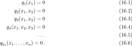
Commutative Gröbner Basis Algorithms can be used to systematically eliminate variables from a collection (e.g., {pj(x1,…,xn) = 0 : 1 ≤ j ≤ k1}) of polynomial equations so as to put it in triangular form. One specifies an order on the variables (x1 < x2 < x3 < … < xn ) 3 which corresponds to ones priorities in eliminating them. Here a GBA will try hardest to eliminate xn and try the least to eliminate x1. The output from it is a list of equations in a “canonical form” which is triangular: 4
In the noncommutative case, again a GB for a collection of polynomial equations is a collection of noncommuting polynomial equations in triangular form (see [HS]). There are some difficulties which don’t occur in the commutative case. For example, a GB can be infinite in the noncommutative case. However, we present software here based on the noncommutative GBA which might prove to be extremely valuable in some situations.
We wish to stress that one does not need to know a theorem in order to discover it using the techniques in this paper. Any method which assumes that all of the hypotheses can be stated algebraically and that all of the hypotheses are known at the beginning of the computation will be of limited practical use. For example, since the Gröbner Basis algorithm only discovers polynomial equations which are algebraically true and not those which require analysis or topology, the use of this algorithm alone has a limited use. Insights gained from analysis during a computer session could be added as (algebraic) hypotheses while the session is in progress. Decisions can take a variety of forms and can involve recognizing a Riccati equation, recognizing that a particular square matrix is onto and so invertible, recognizing that a particular theorem now applies to the problem, etc. The user would then have to record and justify these decisions independently of the computer run. 5 While a strategy allows for human intervention, the intervention must follow certain rigid rules for the computer session to be considered a strategy.
The idea of a prestrategy is :
The above listing is, in fact, a statement of a 1-prestrategy. Sometimes one needs a 2-prestrategy in that the key is equations in 2 unknowns.
The point is to isolate and to minimize what the user must do. This is the crux of a prestrategy.
The prestrategy described above is a loop and we now discuss when to exit the loop.
The digested equations (those in items O1, O2 and O3) often contain the necessary conditions of the desired theorem and the main flow of the proof of the converse. If the starting polynomial equations follow as algebraic consequences of the digested equations, then we should exit the above loop. The starting equations, say {p1 = 0,…,pk1 = 0}, follow as algebraic consequences of the digested equations, say {q1 = 0,…,qk2 = 0}, if and only if the Gröbner Basis generated by {q1,…,qk2} reduces (in a standard way) the polynomial pj to 0 for 1 ≤ j ≤ k1. Checking whether or not this happens is a purely mechanical process.
When one exits the above loop, one is presented with the question of how to finish off the proof of the theorem. We shall call the steps required to go from a final spreadsheet to the actual theorem the “end game.” We shall describe some “end game” technique in §16.3.4. We shall illustrate the “end game” in §14.4 and §17.4. As we shall see, typically the first step is to run NCProcess2 whose output is a very small set of equations.
We mentioned earlier that NCProcess uses the Gröbner Basis algorithm. This GBA is implemented via the command NCMakeGB. If NCProcess consisted of a call to the GBA and the formatted output (§15.2) alone, then NCProcess would not be a powerful enough tool to generate solutions to engineering or math problems. This is because it would generate too many equations. It is our hope that the equations which it generates contain all of the equations essential to solution of whatever problem you are treating. For the problems we have considered, this has been our experience. On the other hand, it contains equations derived from these plus equations derived from those derived from these as well as precursor equations which are no longer relevant. That is, a GB contains a few jewels and lots of garbage. In technical language a GB is almost never a small basis for an ideal and what a human seeks in discovering a theorem is a small basis for an ideal. 6 Thus we have algorithms and substantial software for finding small (or smallest) sets of equations associated to a problem. The process of running GBA followed by an algorithm for finding small sets of equations is what constitutes NCProcess.
We have just given the basic ideas. As a prestrategy proceeds, more and more equations are
digested by the user and more and more unknowns become knowns. Thus we ultimately have two
classes of knowns: original knowns  0 and user designated knowns U. Often a theorem can be
produced directly from the output by taking as hypotheses the existence of knowns U ∪0 which
are solutions to the equations involving only knowns.
0 and user designated knowns U. Often a theorem can be
produced directly from the output by taking as hypotheses the existence of knowns U ∪0 which
are solutions to the equations involving only knowns.
Assume that we have found these solutions. To prove the theorem, that is to construct solutions to the original equations, we must solve the remaining equations. Fortunately, the digested equations often are in a block triangular form which is amenable to backsolving. This is one of the benefits of “digesting” the equations.
An example, makes all of this more clear.
A strategy is like a prestrategy except in addition the user can make (and the program prompts ) certain changes of variables. The nature of these changes of variables is explained in [HS99] and sketched in Chapter 31. The NCProcess output prompts for changes of variables if NCCOV → True by placing parentheses in carefully selected places. The experimental commands described in §31 actually automate this change of variable business to some extent.