
In this section we give a more extensive example of a strategy. For more information of strategies, see [HS]. The command NCCollectOnVariables is an extremely useful command which “collects” knowns and products of knowns out of expressions. For example, suppose that A and B are knowns and X,Y and Z are unknowns. The collected form of
The demonstration in this section will repeatedly call the NCProcess commands with the option NCCV->True (which is the default). This displays formulas in the spreadsheet in an informative way. Whenever a “collected” form of a polynomial is found, the NCProcess command displays it in the collected form rather than as a rule.
A basic problem in systems engineering is to make a given system dissipative by designing a feedback law. We now give a demonstration of how one discovers the algebraic part of the solution to this problem. The following section is reasonably self-contained.
Let Hxx, Hxz, Hzx and Hzz be defined as follows.
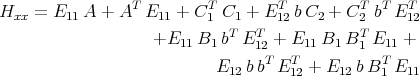
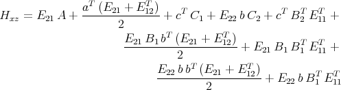
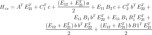
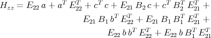
The math problem we address is:
(HGRAIL)
| Let A, B1, B2, C1, C2 be matrices of compatible size be given. Solve Hxx = 0, Hxz = 0, Hzx = 0, and Hzz = 0 for a, b, c and for E11, E12, E21 and E22. When can they be solved? If these equations can be solved, find formulas for the solution. |
The first step is to assemble all of the key relations in executable form:
We make the strong assumption that each Eij is invertible. While this turns out to be valid, making it at this point is cheating. Ironically we recommend strongly that the user make heavy invertibility assumptions at the outset of a session. Later after the main ideas have been discovered the user can selectively relax them and thereby obtain more general results.
Also, the 2 x 2 matrix (Eij) 1 ≤ i,j ≤ 2 is symmetric.
It is a good idea to create an input file for the strategy session before starting Mathematica. There are several preliminary steps which may have to be done several times before the desired results are obtained. Setting the monomial order, setting variables noncommutative and defining the starting equations can all be done beforehand. This way, if the user wants to try the same run with a slightly different ordering, he only needs to edit the input file and load it again.
In this case, the input file is called cntrl. Notice that we are using Tp[ ] to denote transpose and Inv[] to denote inverse, which is inconsistent with the NCAlgebra package which uses tp[ ] and inv[ ] respectively. This is done intentionally to ensure that actual transposes and inverses are not taken within the GBA. The relations can be easily converted later if it is necessary to do mathematical operations on them.
This is the file “cntrl”:
SetNonCommutative[E11,E22,E12,E21,Inv[E11],Inv[E22],Inv[E12],Inv[E21],
Tp[Inv[E11]],Tp[Inv[E22]],Tp[Inv[E12]],Tp[Inv[E21]], Tp[E11],Tp[E22],Tp[E12],Tp[E21]]; (* These relations imply that the Eij generate a symmetric quadratic form. *) transE = { Tp[E21]-E12, Tp[E11]-E11, Tp[E22]-E22, Tp[E12]-E21, Tp[Inv[E21]]-Inv[E12], Tp[Inv[E11]]-Inv[E11], Tp[Inv[E22]]-Inv[E22], Tp[Inv[E12]]-Inv[E21]}; (* These relations assume that everything is invertible *) inverseE = { E11**Inv[E11] -1, Inv[E11]**E11 -1, E12**Inv[E12] -1, Inv[E12]**E12 -1, E21**Inv[E21] -1, Inv[E21]**E21 -1, E22**Inv[E22] -1, Inv[E22]**E22 -1, Tp[E11]**Tp[Inv[E11]] -1, Tp[Inv[E11]]**Tp[E11] -1, Tp[E12]**Tp[Inv[E12]] -1, Tp[Inv[E12]]**Tp[E12] -1, Tp[E21]**Tp[Inv[E21]] -1, Tp[Inv[E21]]**Tp[E21] -1, Tp[E22]**Tp[Inv[E22]] -1, Tp[Inv[E22]]**Tp[E22] -1}; SetNonCommutative[A,Tp[A],B1,Tp[B1],B2,Tp[B2], C1,Tp[C1],C2,Tp[C2], b,Tp[b],c,Tp[c],a,Tp[a]]; (* These are the Hamiltonian equations *) Hxx=E11 ** A + Tp[A] ** Tp[E11] + Tp[C1] ** C1 + Tp[C2] ** Tp[b] ** (E21 + Tp[E12])/2 + (E12 + Tp[E21]) ** b ** C2/2 + E11 ** B1 ** Tp[b] ** (E21 + Tp[E12])/2 + E11 ** B1 ** Tp[B1] ** Tp[E11] + (E12 + Tp[E21]) ** b ** Tp[b] ** (E21 + Tp[E12])/4 + (E12 + Tp[E21]) ** b ** Tp[B1] ** Tp[E11]/2; Hxz=E21 ** A + Tp[a] ** (E21 + Tp[E12])/2 + Tp[c] ** C1 + E22 ** b ** C2 + Tp[c] ** Tp[B2] ** Tp[E11] + E21 ** B1 ** Tp[b]** (E21 + Tp[E12])/2 + E21 ** B1 ** Tp[B1] ** Tp[E11] + E22 ** b ** Tp[b] ** (E21 + Tp[E12])/2 + E22 ** b ** Tp[B1] ** Tp[E11]; Hzx=Tp[A] ** Tp[E21] + Tp[C1] ** c + (E12 + Tp[E21]) ** a/2 + E11 ** B2 ** c + Tp[C2] ** Tp[b] ** Tp[E22] + E11 ** B1 ** Tp[b] ** Tp[E22] + E11 ** B1 ** Tp[B1] ** Tp[E21] + (E12 + Tp[E21]) ** b ** Tp[b] ** Tp[E22]/2 + (E12 + Tp[E21]) ** b ** Tp[B1] ** Tp[E21]/2; Hzz=E22 ** a + Tp[a] ** Tp[E22] + Tp[c] ** c + E21 ** B2 ** c + Tp[c] ** Tp[B2] ** Tp[E21] + E21 ** B1 ** Tp[b] ** Tp[E22] + E21 ** B1 ** Tp[B1] ** Tp[E21] + E22 ** b ** Tp[b] ** Tp[E22] + E22 ** b ** Tp[B1] ** Tp[E21]; Hameq = {Hxx,Hxz,Hzx,Hzz}; (* Set the knowns and the order of the unknowns *) SetKnowns[A,Tp[A],B1,Tp[B1],B2,Tp[B2],C1,Tp[C1],C2,Tp[C2]]; SetUnknowns[E12,Tp[E12],E21,Tp[E21],E22,Tp[E22],E11,Tp[E11], Inv[E12],Tp[Inv[E12]],Inv[E21],Tp[Inv[E21]], Inv[E22],Tp[Inv[E22]],Inv[E11],Tp[Inv[E11]], b,Tp[b],c,Tp[c],a,Tp[a]]; startingrels = Union[transE, inverseE, Hameq]; result1 = NCProcess1[startingrels,2,"cntrlans1"]; |
Now when we load this file, we will be ready to begin the strategy session.
In[1]:= Get["NCGB.m"];
In[2]:= Get["cntrl"]; In[3]:= result1 |
We can ignore the Mathematica output Out[3] of the NCProcess1 command for now. What is important is that the spreadsheet which NCProcess1 produces is in the file “cntrlans1.dvi”. There is no need to record all of it here, since the only work which we must do is on the undigested relations.
When the file “cntrlans1.dvi’ is displayed, the undigested relations are:
_________________________________________________________________________________
____________________ SOME RELATIONS WHICH APPEAR BELOW _____________________________
______________________________ MAY BE UNDIGESTED ___________________________________________
_________________________________________________________________________________
THE FOLLOWING VARIABLES HAVE NOT BEEN SOLVED FOR:
{b,c,E11,E12,E22,E11-1,E12-1,E22-1,bT ,cT ,E12T ,E12-1T }
_________________________________________________________________________________
1.3 The expressions with unknown variables {E11-1,E11}
and knowns {}
| E11 E11-1 → 1 |
| E11-1 E11 → 1 |
| E12 E12-1 → 1 |
| E12-1 E12 → 1 |
| E22 E22-1 → 1 |
| E22-1 E22 → 1 |
| E12T E12-1T → 1 |
| E12-1T E12T → 1 |
| bbT + bC2 E12-1T + E12-1 C2T bT + E12-1 E11 AE12-1T + E12-1 E11 B1 bT + E12-1 AT E11 E12-1T + E12-1 C1T C1 E12-1T + (b + E12-1 E11 B1)B1T E11E12-1T = 0 |
| cT c + cT B2T (E12 - E11 E12-1T E22)-(E22 E12-1 E11-E12T )B2c -E22 E12-1 AT (E12-E11 E12-1T E22) - E22 E12-1 C1T (c - C1 E12-1T E22) - cT C1 E12-1T E22 + (E22 E12-1 E11 - E12T )AE12-1T E22 - (E22 E12-1 E11 - E12T )B1B1T (E12 - E11 E12-1T E22) = 0 |
As we can easily see from the spreadsheet above, there are only two nontrivial relations left undigested by the NCProcess1 command. The user can ignore the rest of the spreadsheet for now. Since the leading terms of the last two polynomials above are bbT and ccT , and the fact that the two equations are decoupled (i.e. the bbT equation does not depend on c or CT and the ccT equation does not depend on b or bT ) further iterations of an NCProcess command would probably not help. At this point, we need to be more clever.
We begin by assigning variables to the polynomials that we are interested in. We can see from Out[3] that the polynomial involving b and Tp[b] is the first element of the third list in the result1, and the c rule is the last element of that list. These relations are in the form of rules which need to be converted to polynomials before we can continue. This is done with the command RuleToPoly. The next step is to convert the Tp[ ] in these rules to tp[ ], which will be recognized as transpose by NCAlgebra. Here is how this is done:
In[4]:= bpoly = RuleToPoly[result1[[3,1]]]
Out[4]:= b ** Tp[b] + b ** C2 ** Inv[E21] + Inv[E12] ** Tp[C2] ** Tp[b] + > b ** Tp[B1] ** E11 ** Inv[E21] + Inv[E12] ** E11 ** A ** Inv[E21] + > Inv[E12] ** E11 ** B1 ** Tp[b] + Inv[E12] ** Tp[A] ** E11 ** Inv[E21] + > Inv[E12] ** Tp[C1] ** C1 ** Inv[E21] + Inv[E12] ** E11 ** B1 ** > Tp[B1] ** E11 ** Inv[E21] In[5]:= cpoly = RuleToPoly[result1[[3,-1]]] Out[5]:= Tp[c] ** c + E21 ** B2 ** c + Tp[c] ** Tp[B2] ** E12 - > E21 ** A ** Inv[E21] ** E22 + E21 ** B1 ** Tp[B1] ** E12 - > E22 ** Inv[E12] ** Tp[A] ** E12 - E22 ** Inv[E12] ** Tp[C1] ** c - > Tp[c] ** C1 ** Inv[E21] ** E22 - E22 ** Inv[E12] ** E11 ** B2 ** c - > Tp[c] ** Tp[B2] ** E11 ** Inv[E21] ** E22 - > E21 ** B1 ** Tp[B1] ** E11 ** Inv[E21] ** E22 + > E22 ** Inv[E12] ** E11 ** A ** Inv[E21] ** E22 - > E22 ** Inv[E12] ** E11 ** B1 ** Tp[B1] ** E12 + > E22 ** Inv[E12] ** Tp[A] ** E11 ** Inv[E21] ** E22 + > E22 ** Inv[E12] ** Tp[C1] ** C1 ** Inv[E21] ** E22 + > E22 ** Inv[E12] ** E11 ** B1 ** Tp[B1] ** E11 ** Inv[E21] ** E22 In[6]:= bpoly = bpoly /. Tp->tp; In[7]:= cpoly = cpoly /. Tp->tp; |
Observe that the polynomials Out[4] is quadratic in b. We could complete the square and get to put the polynomial in the form
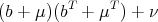
where μ and ν are expressions involving C2, C2T , B 1, B1T , A, AT , E 21-1, E 12-1 and E 11. Since there are many unknowns in the problem, there is probably excess freedom. Let us investigate what happens when we take b + μ = 0. NCAlgebra is very good with quadratics so this is easy to execute, but since this is not a general NCAlgebra tutorial we shall not describe how this is done, but just write down the answer.
Out[8]:= -iE12 ** tp[C2] tp[iE21] ** tp[C2]
b -> --------------- - ------------------ - 2 2 iE12 ** E11 ** B1 tp[iE21] ** tp[E11] ** B1 > ----------------- - ------------------------- 2 2 |
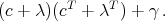
We can also complete the square for the expression in c and put that expression in the form
Out[9]:= -tp[B2] ** E12 tp[B2] ** tp[E21] C1 ** iE21 ** E22
c -> -------------- - ----------------- + ----------------- + 2 2 2 C1 ** tp[iE12] ** tp[E22] tp[B2] ** E11 ** iE21 ** E22 > ------------------------- + ---------------------------- + 2 2 tp[B2] ** tp[E11] ** tp[iE12] ** tp[E22] > ---------------------------------------- 2 |
Next we do some petty bookkeeping to get transposes of the above two rules. Once we have solved for b and c, we can then take the transpose of each of these rules to solve for tp[b] and tp[c]. In our strategy session, these are simply two additional unknowns which we can now eliminate.
In[10]:= bpoly = RuleToPoly[brule];
In[11]:= cpoly = RuleToPoly[crule]; In[12]:= newpolys = {bpoly,cpoly,tp[bpoly],tp[cpoly]}; In[13]:= newrules = PolyToRule[newpolys]; In[14]:= newrules = newrules /. tp->Tp; In[15]:= newrules = newrules /. PolyToRule[transE] Out[15]:= {b -> -iE12 ** Tp[C2] + -iE12 ** E11 ** B1, Tp[b] -> -C2 ** iE21 + -Tp[B1] ** E11 ** iE21, c -> -Tp[B2] ** E12 + C1 ** iE21 ** E22 + Tp[B2] ** E11 ** iE21 ** E22, Tp[c] -> -E21 ** B2 + E22 ** iE12 ** Tp[C1] + E22 ** iE12 ** E11 ** B2} |
In[14] takes these four rules and replaces tp with Tp. In[15] simplifies these equations by making the substitutions for the transposes of E which we have been using. Now we have four additional polynomials which can be added to the input for the next call to NCProcess1.
The starting relations for this step will be the output from the first NCProcess1 call which was result1, as well as the four new equations that we have just derived. Just as we did in the first step, we will create a file to be read in to the Mma session.
This is the file “cntrl2”.
digested=RuleToPoly[result1[[2]]];
undigested=RuleToPoly[result1[[3]]]; relations=Join[digested,newpolys,undigested]; result2=NCProcess1[relations,2,"cntrlans2", DegreeCap->6,DegreeSumCap->9]; |
Now, if we do not like the results, we can change the DegreeCap options or the iteration count and simply read the file again, without typing the entire sequence of commands again. Then in the Mathematica session, we simply type
In[16]:= Get["cntrl2"];
|
Once again we go directly to the file which NCProcess1 created. There is no need to record all of it, since at this stage we shall be concerned only with the undigested relations.
When the file “cntrlans2.dvi” is displayed, the undigested relations are:
_________________________________________________________________________________
____________________ SOME RELATIONS WHICH APPEAR BELOW _____________________________
______________________________ MAY BE UNDIGESTED ___________________________________________
_________________________________________________________________________________
THE FOLLOWING VARIABLES HAVE NOT BEEN SOLVED FOR:
{E11,E12,E22,E11-1,E12-1,E22-1,E12T ,E12-1T }
_________________________________________________________________________________
1.0 The expressions with unknown variables {E11}
and knowns {A,B1,C1,C2,AT ,B1T ,C1T ,C2T }
| E11 B1 C2 → E11 A + AT E11 + C1T C1 - C2T C2 - C2T B1T E11 |
| E11 E11-1 → 1 |
| E11-1 E11 → 1 |
| E12 E12-1 → 1 |
| E12-1 E12 → 1 |
| E22 E22-1 → 1 |
| E22-1 E22 → 1 |
| E12T E12-1T → 1 |
| E12-1T E12T → 1 |
| E22 E12-1 AT (E12 - E11 E12-1T E22) - (E22 E12-1 E11 - E12T )AE12-1T E22 + (E22 E12-1 E11 - E12T )B1B1T (E12 - E11 E12-1T E22) - (E22 E12-1 E11 - E12T )B2B2T (E12 - E11 E12-1T E22) - E22 E12-1 C1T B2T (E12 - E11 E12-1T E22) + (E22 E12-1 E11 - E12T )B2C1 E12-1T E22 = 0 |
Once again, we have two equations worth looking at.
The first polynomial equation is a (Riccati-Lyapunov) equation in E11. Numerical methods for solving Riccati equations are common. For this reason assuming that a Riccati equation has a solution is a socially acceptable necessary condition throughout control engineering. Thus we can consider E11 to be known.
We notice that the same products of unknowns appear over and over. It is likely that we can factor or group this equation in such a way that we can understand it a little better.
We start by grabbing the relation which we want to explore. Although the spreadsheet above shows the equation in factored form, it is returned to Mathematica in expanded form. In this case, the relation we are interested in is the thirteenth element in the third list of result2.
In[18] := equ2 = result2[[3,13]] Out[18]= E22 ** Inv[E12] ** Tp[A] ** E12 + > Tp[E12] ** A ** Tp[Inv[E12]] ** E22 - Tp[E12] ** B1 ** Tp[B1] ** E12 + > Tp[E12] ** B2 ** Tp[B2] ** E12 - > E22 ** Inv[E12] ** Tp[C1] ** Tp[B2] ** E12 - > Tp[E12] ** B2 ** C1 ** Tp[Inv[E12]] ** E22 - > E22 ** Inv[E12] ** E11 ** A ** Tp[Inv[E12]] ** E22 + > E22 ** Inv[E12] ** E11 ** B1 ** Tp[B1] ** E12 - > E22 ** Inv[E12] ** E11 ** B2 ** Tp[B2] ** E12 - > E22 ** Inv[E12] ** Tp[A] ** E11 ** Tp[Inv[E12]] ** E22 + > Tp[E12] ** B1 ** Tp[B1] ** E11 ** Tp[Inv[E12]] ** E22 - > Tp[E12] ** B2 ** Tp[B2] ** E11 ** Tp[Inv[E12]] ** E22 + > E22 ** Inv[E12] ** E11 ** B2 ** C1 ** Tp[Inv[E12]] ** E22 + > E22 ** Inv[E12] ** Tp[C1] ** Tp[B2] ** E11 ** Tp[Inv[E12]] ** E22 - > E22 ** Inv[E12] ** E11 ** B1 ** Tp[B1] ** E11 ** Tp[Inv[E12]] ** E22 + > E22 ** Inv[E12] ** E11 ** B2 ** Tp[B2] ** E11 ** Tp[Inv[E12]] ** E22 |
Now we can see from the factored form in the spreadsheet that this equation is symmetric. It would not take an experienced mathematician long to realize that by multiplying this equation on the left by E12 E22-1 and on the right by E 22-1 E 21, we will have an equation in one unknown.
In[19]:= equ3 = NCExpand[E12**Inv[E22]**equ2**Inv[E22]**E21];
|
Inspection of equ3 shows that the following valid substitution would be helpful.
In[20]:= equ4 = Transform[equ3,
{Inv[E22]**E22->1,E12**Inv[E12]->1,E22**Inv[E22]->1,Inv[E21]**E21->1}]; |
We now obtain the collected form of equ4.
In[21]:= equ5 = NCCollectOnVariables[equ4]
Out[21]:= -(E11 - E12 ** Inv[E22] ** E21) ** A - > Tp[A] ** (E11 - E12 ** Inv[E22] ** E21) + > (E11 - E12 ** Inv[E22] ** E21) ** B2 ** C1 + > Tp[C1] ** Tp[B2] ** (E11 - E12 ** Inv[E22] ** E21) - > (E11 - E12 ** Inv[E22] ** E21) ** B1 ** Tp[B1] ** (E11 - E12 ** Inv[EE22] ** E21) + > (E11 - E12 ** Inv[E22] ** E21) ** B2 ** Tp[B2] ** (E11 - E12 ** Inv[E22] ** E21) |
Now we can replace E11 - E12 E22-1 E 21 with a new variable X.
In[22]:= Transform[equ5,(E11 - E12 ** Inv[E22] ** E21)->X]
Out[22]:= -X ** A - Tp[A] ** X + X ** B2 ** C1 + Tp[C1] ** Tp[B2] ** X - > X ** B1 ** Tp[B1] ** X + X ** B2 ** Tp[B2] ** X |
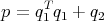
Observe that this is an equation in the one unknown X. Of course, the only other undigested equation was in the one unknown E11 and the previous spreadsheet featured an equation in the single unknown b (and its transpose) and an equation in the single unknown c (and its transpose). Thus we have solved (HGRAIL) with a symmetrized liberalized 2-strategy (see [HS]).
Now let us compare what we have found to the well known solution of (HGRAIL). In that theory there are two Riccati equations due to Doyle, Glover, Khargonekar and Francis. These are the DGKF X and Y equations. One can read off that the E11 equation which we found is the DGKF equation for Y -1, while the Riccati equation which we just analyzed is the DGKF X equation.
Indeed what we have proved is that if (HGRAIL) has a solution with Eij invertible and if b and c are given by formulas Out[8] and Out[9] in §17.3.2, then
Now we turn to the converse. The straightforward converse of the above italicized statement would be: If items (1), (2) and (3) above hold, then (HGRAIL) has a solution with Eij invertible and b and c are given by formulas Out[8] and Out[9] in §17.3.2. There is no reason to believe (and it is not the case) that b and c must be given by the formulas Out[8] and Out[9] in §17.3.2. These two formulas came about in §17.3.2 and were motivated by “excess freedom” in the problem. The converse which we will attempt to prove is:
Proposed Converse 17.1 If items (1), (2) and (3) above hold, then (HGRAIL) has a solution with Eij invertible.
To obtain this proposed converse, we need a complete spreadsheet corresponding to the last stages of our analysis. The complete spreadsheet is:
THE ORDER IS NOW THE FOLLOWING:
A < AT < B1 < B1T < B2 < B2T < C1 < C1T < C2 < C2T < X < X-1 < Y < Y -1 ≪ E12 ≪ E21 ≪ E22 ≪ E12T ≪ E21T ≪
E22T ≪ E11 ≪ E11T ≪ E11-1 ≪ E11-1T ≪ E12-1 ≪ E21-1 ≪ E22-1 ≪ E12-1T ≪ E21-1T ≪ E22-1T ≪ b ≪ bT ≪ c ≪ cT ≪ a ≪ aT
_________________________________________________________________________________
__________________________ YOUR SESSION HAS DIGESTED _____________________________________
__________________________ THE FOLLOWING RELATIONS ______________________________________
_________________________________________________________________________________
THE FOLLOWING VARIABLES HAVE BEEN SOLVED FOR:
{a,b,c,E11,E11-1,aT ,bT ,cT ,E11T ,E12T ,E21T ,E22T ,E11-1T ,E12-1T ,E21-1T ,E22-1T }
The corresponding rules are the following:
| a →-E12-1 AT E12+E12-1 C1T B2T E12+E12-1 C2T B1T E12+E12-1 E11 B2 B2T E12- E12-1 C1T C1 E21-1 E22 -E12-1 E11 B2 C1 E21-1 E22 -E12-1 C1T B2T E11 E21-1 E22 - E12-1 E11 B2 B2T E11 E21-1 E22 |
| b →-E12-1 C2T - E12-1 E11 B1 |
| c →-B2T E12 + C1 E21-1 E22 + B2T E11 E21-1 E22 |
| E11 → Y -1 |
| E11-1 → Y |
| aT → -E21 AE21-1 + E21 B1 C2 E21-1 + E21 B2 C1 E21-1 + E21 B2 B2T E11 E21-1 - E22 E12-1 C1T C1 E21-1 -E22 E12-1 E11 B2 C1 E21-1 -E22 E12-1 C1T B2T E11 E21-1 - E22 E12-1 E11 B2 B2T E11 E21-1 |
| bT →-C2 E21-1 - B1T E11 E21-1 |
| cT →-E21 B2 + E22 E12-1 C1T + E22 E12-1 E11 B2 |

| X X-1 → 1 |
| Y Y -1 → 1 |
| X-1 X → 1 |
| Y -1 Y → 1 |
| Y -1 B1 C2 → Y -1 A + AT Y -1 + C1T C1 - C2T C2 - C2T B1T Y -1 |
| X B2 B2T X → X A + AT X - X B2 C1 - C1T B2T X + X B1 B1T X |
| E11-1 → Y |
| E12 E22-1 E21 → E11 - X |
| E12 E12-1 → 1 |
| E12-1 E12 → 1 |
| E21 E21-1 → 1 |
| E21-1 E21 → 1 |
| E22 E22-1 → 1 |
| E22-1 E22 → 1 |
| ⇑ E12 E22-1 E21 → E11 - X |
In the spreadsheet, we use conventional X, Y -1 notation rather than “discovered” notation so that our arguments will be familiar to experts in the field of control theory.
Now we use the above spreadsheet to verify the proposed converse. To do this, we assume that matrices A, B1, B2, C1, C2, X and Y exist, that X and Y are invertible, that X and Y are self-adjoint, that Y -1 - X is invertible and that the DGKF X and Y -1 equations hold. That is, the two following polynomial equations hold.
Y -1 B
1 C2 = Y -1 A + AT Y -1 + C
1T C
1 - C2T C
2 - C2T B
1T Y -1
X B2 B2T X = X A + AT X - X B
2 C1 - C1T B
2T X + X B
1 B1T X
We wish to assign values for the matrices E12, E21, E22, E11, a, b and c such that each of the equations on the above spreadsheet hold. If we can do this, then each of the equations from the starting polynomial equations from §17.1 will hold and the proposed converse will follow.
With the assignments of E12, E21, E22, E11, a, b and c as above, it is easy to verify by inspection that every polynomial equation on the spreadsheet above holds.
We have proven the proposed converse and, therefore, have proven the following approximation to the classical [DGKF] theorem.
Theorem 17.2 If (HGRAIL) has a solution with invertible Eij and b and c are given by the formulas Out[8] and Out[9] in §17.3.2, then the DGKF X and Y -1 equations have solutions X and Y which are symmetric matrices with X,Y -1 and Y -1 - X invertible. The DGKF X and Y -1 equations have solutions X and Y which are symmetric matrices with X,Y -1 and Y -1 - X invertible, then (HGRAIL) has a solution with invertible E ij.
Note that we obtained this result with an equation in the one unknown X and an equation with the one unknown E11 = Y -1. From the strategy point of view, the first spreadsheet featured an equation in the single unknown b (and its transpose) and an equation in the single unknown c (and its transpose) and so is the most complicated. For example, the polynomial Out[4] in §17.3.2 decomposes as
 | (17.3) |
where q1 = b + E12-1 C 2T + E 12-1 E 11 B1 and q2 is a symmetric polynomial which does not involve b. This forces us to say that the proof of the necessary side of Theorem 17.2 was done with a 2-strategy.
A more aggressive way of selecting knowns and unknowns allows us to obtain this same result with a symmetrized 1-strategy. In particular, one would set a, b and c to be the only unknowns to obtain a first spreadsheet. The first spreadsheet contains key equations like (17.3), which is a symmetric 1-decomposition, because q2 does not contain a, b or c. Once we have solved for a, b and c, we turn to the next spreadsheet by declaring the variables involving Eij (e.g., E11, E11-1, . . . ) to be unknown. At this point, the computer run is the same as Steps 2, 3 and 4 above.