5 Continuous Distributions
5.1 Uniform distributions
Here are the density, (cumulative) distribution function, survival function, and quantile function of the uniform distribution on \([0,1]\)
x = seq(-0.2, 1.2, len = 1000)
u = seq(0, 1, len = 1000)
par(mfrow = c(2,2), mai = c(0.35, 0.35, 0.1, 0.1))
plot(x, dunif(x), type = "l", lwd = 2, ylab = "", xlab = "")
plot(x, punif(x), type = "l", lwd = 2, ylab = "", xlab = "")
plot(x, 1-punif(x), type = "l", lwd = 2, ylab = "", xlab = "")
plot(u, qunif(u), type = "l", lwd = 2, ylab = "", xlab = "")
abline(v = c(0, 1), lty = 2)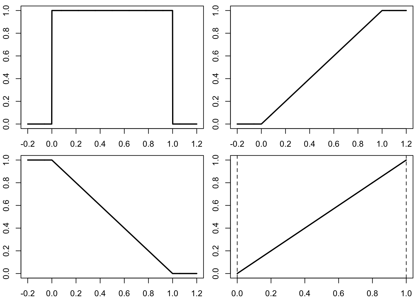
5.2 Normal distributions
Here are the density, (cumulative) distribution function, survival function, and quantile function of the standard normal distribution (mean 0, variance 1)
x = seq(-3, 3, len = 1000)
par(mfrow = c(2,2), mai = c(0.35, 0.35, 0.1, 0.1))
plot(x, dnorm(x), type = "l", lwd = 2, ylab = "", xlab = "")
plot(x, pnorm(x), type = "l", lwd = 2, ylab = "", xlab = "")
plot(x, 1-pnorm(x), type = "l", lwd = 2, ylab = "", xlab = "")
plot(u, qnorm(u), type = "l", lwd = 2, ylab = "", xlab = "")
abline(v = c(0, 1), lty = 2)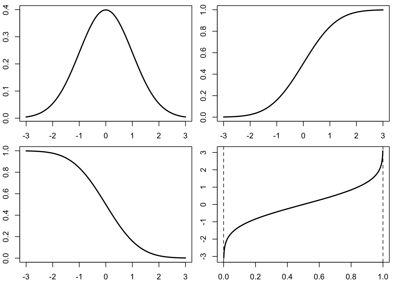
5.3 Exponential distributions
Here are the density, (cumulative) distribution function, survival function, and quantile function of the exponential distribution with rate 1
x = seq(-1, 5, len = 1000)
par(mfrow = c(2,2), mai = c(0.35, 0.35, 0.1, 0.1))
plot(x, dexp(x), type = "l", lwd = 2, ylab = "", xlab = "")
plot(x, pexp(x), type = "l", lwd = 2, ylab = "", xlab = "")
plot(x, 1-pexp(x), type = "l", lwd = 2, ylab = "", xlab = "")
plot(u, qexp(u), type = "l", lwd = 2, ylab = "", xlab = "")
abline(v = c(0, 1), lty = 2)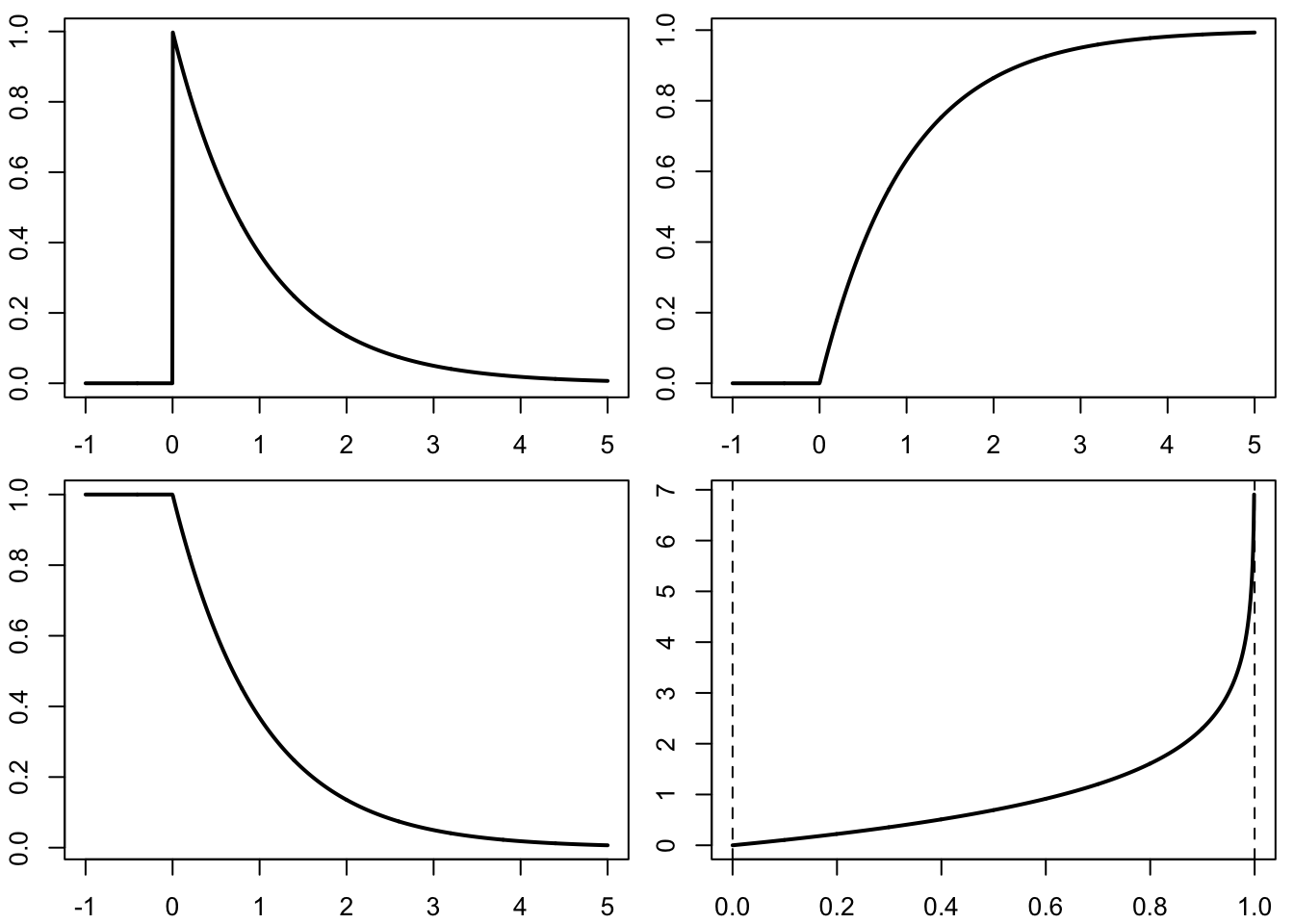
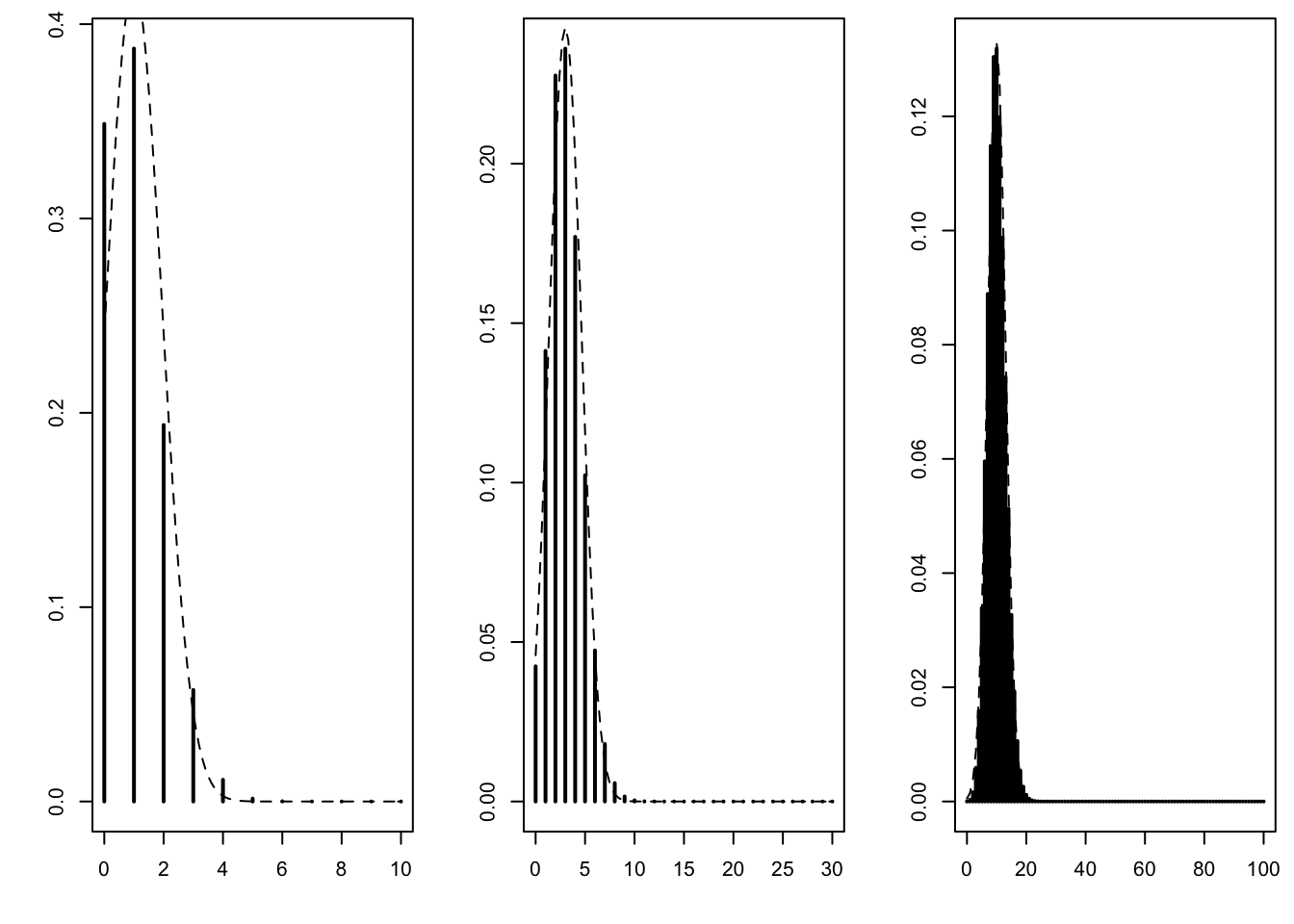
5.4 Normal approximation to the binomial
The de Moivre–Laplace theorem says that, as \(n\) increases while \(p\) remains fixed, the binomial distribution with parameters \((n, p)\) is well approximated by the normal distribution with same mean (\(= np\)) and same variance (\(= n p (1-p)\)). To verify this numerically, we fix \(p = 0.10\) and vary \(n\) in \(\{10, 30, 100\}\). We can see that the approximation is already very good when \(n = 100\).
par(mfrow = c(1, 3), mai = c(0.5, 0.5, 0.1, 0.1))
n = 10
p = 0.1
plot(0:n, dbinom(0:n, n, p), type = "h", lwd = 2, xlab = "", ylab = "")
curve(dnorm(x, n*p, sqrt(n*p*(1-p))), add = TRUE, lty = 2)

n = 30
p = 0.1
plot(0:n, dbinom(0:n, n, p), type = "h", lwd = 2, xlab = "", ylab = "")
curve(dnorm(x, n*p, sqrt(n*p*(1-p))), add = TRUE, lty = 2)

n = 100
p = 0.1
plot(0:n, dbinom(0:n, n, p), type = "h", lwd = 2, xlab = "", ylab = "")
curve(dnorm(x, n*p, sqrt(n*p*(1-p))), add = TRUE, lty = 2)