12 Models, Estimators, and Tests

12.1 Confidence intervals

A confidence interval is a random interval, that is, before it is numerically evaluated on observed data. (It is a function of the data, which are modeled as random.) It is not guaranteed to contain the true value of the parameter of interest — the parameter the interval is built for — but only contains it with some probability equal to its coverage, which is controlled by the confidence level when the construction of the interval is properly calibrated. To illustrate this, we consider the Clopper–Pearson two-sided confidence interval for the probability parameter of a binomial distribution. (The number of trials defining the binomial distribution is fixed in what follows.)

n = 20 # number of trials
theta = 0.3 # probability parameter
B = 100 # number of replicates
L = numeric(B) # storing the lower bound of the interval
U = numeric(B) # storing the upper bound of the interval
Y = rbinom(B, n, theta) # simulated data with each number corresponding to one replicate
for (b in 1:B){
  test = binom.test(Y[b], n, conf = 0.90)
  L[b] = test$conf.int[1]
  U[b] = test$conf.int[2]
}
plot(0, 0, type = "n", xlim = c(0, 1), ylim = c(0, B), xlab = "Intervals", ylab = "Experiments", cex.lab = 1)
segments(L, 1:B, U, 1:B, col = "darkgrey")
abline(v = theta, col = "darkred") # indicates the true value of the parameter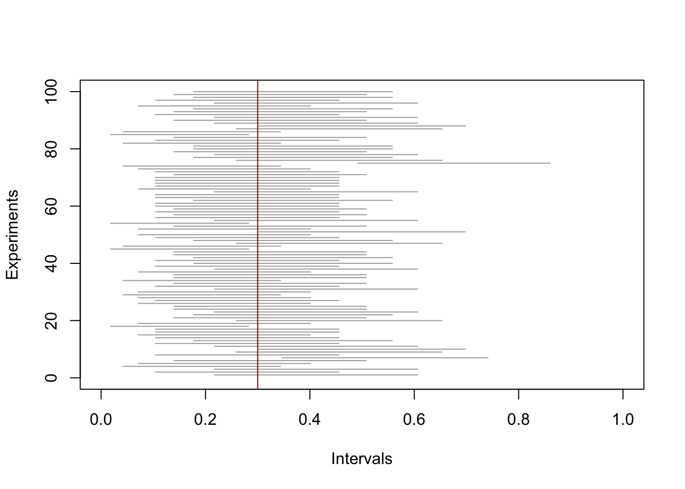

While the target level was 90 percent, the interval contained the true value of the parameter the following fraction of times

mean((L < theta)*(U > theta))

[1] 0.91

12.2 Tests

Similarly, the outcome of a test is random, that is, before it is numerically evaluated on observed data. The probability of rejecting by mistake (a Type I error) is the size of the test, which is controlled by the level when the test is properly calibrated. In the same context of a binomial experiment with parameters \((\theta, n)\), with \(n\) given, the likelihood ratio test for the null hypothesis \(\theta \le \theta_0\) rejects for large values of \(Y\), the number of heads. (This test corresponds to a one-sided Clopper–Pearson confidence interval.) Suppose \(\theta_0 = 1/2\) and that we are testing at the \(\alpha = 0.10 = 10\%\) level. The critical value is given by \[c = \min\{c': \mathbb{P}_{1/2}(Y \le c') \ge 1-\alpha\},\] which is here equal to

n = 20
alpha = 0.10
(c = qbinom(1-alpha, n, 1/2))

[1] 13

pbinom((c-1):(c+1), n, 1/2)

[1] 0.8684120 0.9423409 0.9793053

The effective size of the test \(\{Y > c\}\) is \(\mathbb{P}_{1/2}(Y > c)\), here equal to

1 - pbinom(c, n, 1/2) 

[1] 0.05765915

It is bounded from above by \(\alpha\) by construction, and in fact, quite a bit smaller in this particular case, so that the test is quite conservative. (Note that the test can also be performed using the function binom.)

Let’s evaluate the power of this test against various alternatives.

theta = seq(1/2, 1, len = 10) # range for the probability parameter
B = 100 # number of replicates
test = matrix(NA, B, length(theta)) # rows: replicates; columns: values of theta
for (i in 1:length(theta)){
  Y = rbinom(B, n, theta[i])
  for (b in 1:B){
    test[b, i] = (Y[b] > c)
  }
}
power = colMeans(test) # empirical power
plot(theta, power, type = "b", lwd = 2, ylim = c(0,1), xlab = paste("true probability parameter"), ylab = "fractions of rejections", cex.lab = 1)
abline(h = alpha, lty = 2) # indicates the desired level
abline(h = 1, lty = 2) # indicates full power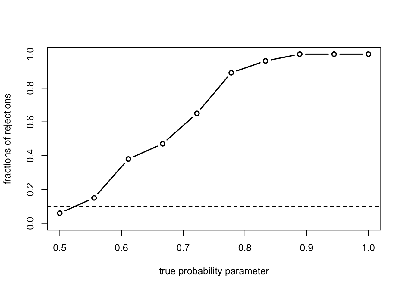

In accord with theory, we see that the power at \(\theta = \theta_0 = 1/2\), which falls within the null hypothesis, is below \(\alpha = 0.10\), and the (empirical) power increases as \(\theta\) increases, moving progressively further away from the null set. Note that the test seems to reach full power at around \(\theta = 0.9\), although the power is, in fact, never equal to 1 in the present situation.