17 Multiple Numerical Samples
17.1 An example of A/B testing
The modern name for two-sample comparison is “A/B testing”. This terminology is particularly prevalent in the high-tech industry. The following is an example of that appearing in Kaggle (https://www.kaggle.com/yufengsui/mobile-games-ab-testing) and DataCamp (https://www.datacamp.com/projects/184). Summarizing the description provided on Kaggle, Cookie Cats is a mobile puzzle game. As a players progress through the levels of the game, they will occasionally encounter gates that force them to wait a non-trivial amount of time or make an in-app purchase to progress. In addition to driving in-app purchases, these gates serve the important purpose of giving players an enforced break from playing the game, hopefully resulting in the player’s enjoyment of the game being increased and prolonged. But where should the gates be placed? In the present experiment, the effects of placing the first gate at level 30 and level 40 are compared, in particular in terms of player retention. Here are the variables:- userid: player identifier
- version: level where the first gate appeared (for that player)
- sum_gamerounds: number of game rounds played (by that player) during the first week after installation
- retention_1: did the player come back and play 1 day after installing?
- retention_7: did the player come back and play 7 days after installing?
load("data/cookie_cats.rda")We focus on the number of game rounds played in the first week after installation. (We are only interested in the 2nd and 3rd variables. We rename the latter for convenience.)
attach(cookie_cats)
rounds = sum_gamerounds
17.1.1 Boxplots
Comparing the plots below (original scale, and then log scale), we see that the values are of very different orders of magnitude, and because of that, the data are more clearly rendered in log scale.
par(mfrow = c(2,1), mai = c(0.5, 0.5, 0.1, 0.1))
boxplot(rounds ~ version, range = Inf, col = 2:3, horizontal = TRUE, xlab = "number of rounds", ylab = "version")
boxplot(log(rounds + 1) ~ version, range = Inf, col = 2:3, horizontal = TRUE, xlab = "number of rounds (log scale)", ylab = "version")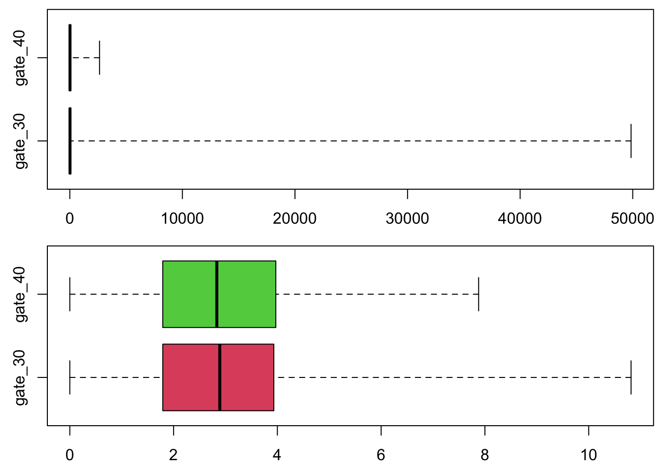
So we work with a log scale henceforth
rounds = log(rounds + 1)17.1.2 Histograms
rounds40 = rounds[version == "gate_40"]
rounds30 = rounds[version == "gate_30"]
par(mfrow = c(2,1), mai = c(1, 1, 0.2, 0.2))
hist(rounds40, breaks = 50, xlim = range(rounds), main = "", xlab = "log number of rounds with gate at 40", las = 1, col = 3)
hist(rounds30, breaks = 50, xlim = range(rounds), main = "", xlab = "log number of rounds with gate at 30", las = 1, col = 2)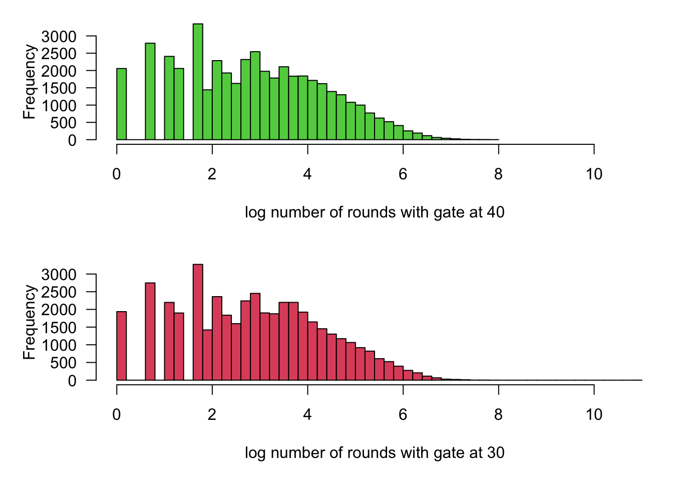
17.1.3 Welch–Student test
To compare the two means, we simply apply the two-sample Welch–Student test. (The samples are quite large and after applying a log transformation their distributions are not overly skewed or heavy-tailed, which is reassuring when applying this test.) The function also computes the related confidence interval for the difference in means.
t.test(rounds30, rounds40)
    Welch Two Sample t-test

data:  rounds30 and rounds40
t = 1.8142, df = 90177, p-value = 0.06964
alternative hypothesis: true difference in means is not equal to 0
95 percent confidence interval:
 -0.001459544  0.037796681
sample estimates:
mean of x mean of y
 2.888910  2.870742
There is some evidence that with the first gate shown at level 30 a player will play more rounds (at least in the first week after installing the game).
17.1.4 Rank tests
We apply Wilcoxon rank-sum test and the Kolmogorov–Smirnov test. (Each of these is a rank test, and any rank test returns the same p-value regardless of whether it is applied before or after transformation.)
wilcox.test(rounds30, rounds40)
    Wilcoxon rank sum test with continuity correction

data:  rounds30 and rounds40
W = 1024331250, p-value = 0.05021
alternative hypothesis: true location shift is not equal to 0ks.test(rounds30, rounds40)
    Two-sample Kolmogorov-Smirnov test

data:  rounds30 and rounds40
D = 0.010271, p-value = 0.01719
alternative hypothesis: two-sided
Again, there is some evidence that the two samples do not come from the same distribution. (There are some ties in the data, and that impedes the second function from returning the exact p-value, which is computed recursively based on combinatorial identities that are only applicable when all the observations are distinct.) In any case, although somewhat statistically significant, the difference may not be meaningful as it is quite small. (The median number of rounds played differs by just 1.)