9 Stochastic Processes
9.1 Markov chains
We start with a two-state Markov chain with transition matrix
a = 0.5 # probability of staying in state 1
b = 0.1 # probability of staying in state 2
Theta = matrix(c(a, 1-b, 1-a, b), 2, 2) # transition matrix
n = 10 # number of states
x = integer(n+1) # successive states
x[1] = sample(1:2, 1) # starting state drawn uniformly at random
for (i in 1:n){
  x[i+1] = ifelse(x[i] == 1, sample(1:2, prob = c(a, 1-a)), sample(1:2, prob = c(1-b, b)))
}
print(x)
[1] 1 1 2 1 1 1 1 2 1 2 1plot(0:n, x, type = "b", pch = 15, lty = 2, xlab = "time", ylab = "state", axes = FALSE)
axis(1, at = 0:n)
axis(2, at = 1:2)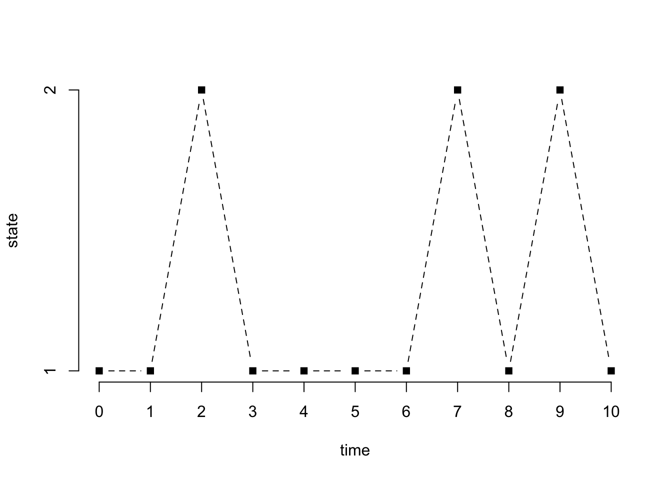
We now use a package which allows for the definition of Markov chain objects. We define the same Markov chain (same transition matrix), but change the states to \(A\) and \(B\) (instead of 1 and 2).
require(markovchain)
MC = new("markovchain", states = c("A", "B"), transitionMatrix = Theta)
plot(MC)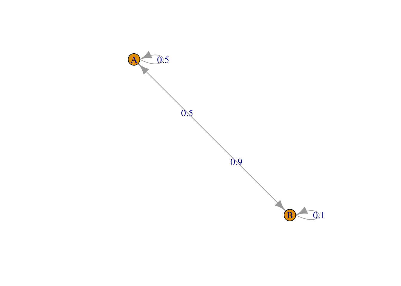
The following generates a sample of size \(n\) from the chain starting at a state that is generated uniformly at random (which is the default)
x = rmarkovchain(n+1, MC)
print(x, quote = FALSE)
[1] A A B A B A B A B B Ax[x == "A"] = 1
x[x == "B"] = 2
plot(0:n, x, type = "b", pch = 15, lty = 2, xlab = "time", ylab = "state", axes = FALSE)
axis(1, at = 0:n)
axis(2, at = 1:2, labels = c("A", "B"))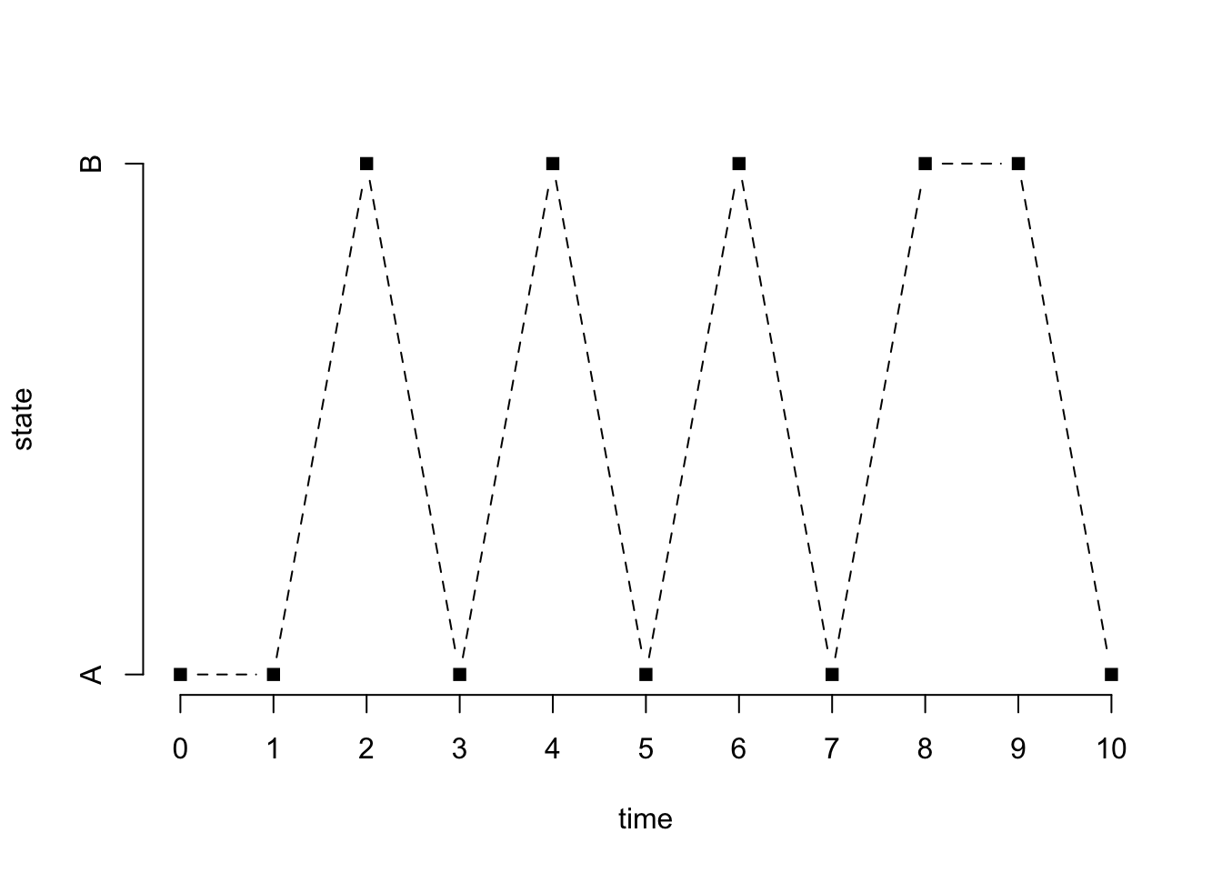
An irreducible, aperiodic, and positively recurrent Markov chain has a unique stationary distribution given by the (unique) left eigenvector of the transition matrix for the eigenvalue 1. The chain above satisfies these properties, and its stationary distribution is the following
out = eigen(t(Theta)) # note the transpose
out = out$vec[, 1] # eigenvector
q = as.vector(out)/sum(out) # normalized so the entries sum to 1
names(q) = c("A", "B")
print(q)
A B
0.6428571 0.3571429 We can verify the theory by running the chain for a long time while recording the fraction of time the run spends in each state
n = 1e3
x = rmarkovchain(n, MC, t0 = "A") # starting from A
table(x)/n
x
A B
0.651 0.349 x = rmarkovchain(n, MC, t0 = "B") # starting from B
table(x)/nx
A B
0.637 0.363 9.2 Simple random walk
A (symmetric) simple random walk is, in a sense, a Markov chain with states \(\{-1, 1\}\), except that the focus is on the partial sums
n = 1e4 # length of the walk
x = sample(c(-1,1), n, replace = TRUE)
s = c(0, cumsum(x)) # partial sums
plot(0:n, s, type = "l", lwd = 2, xlab = "step", ylab = "partial sum")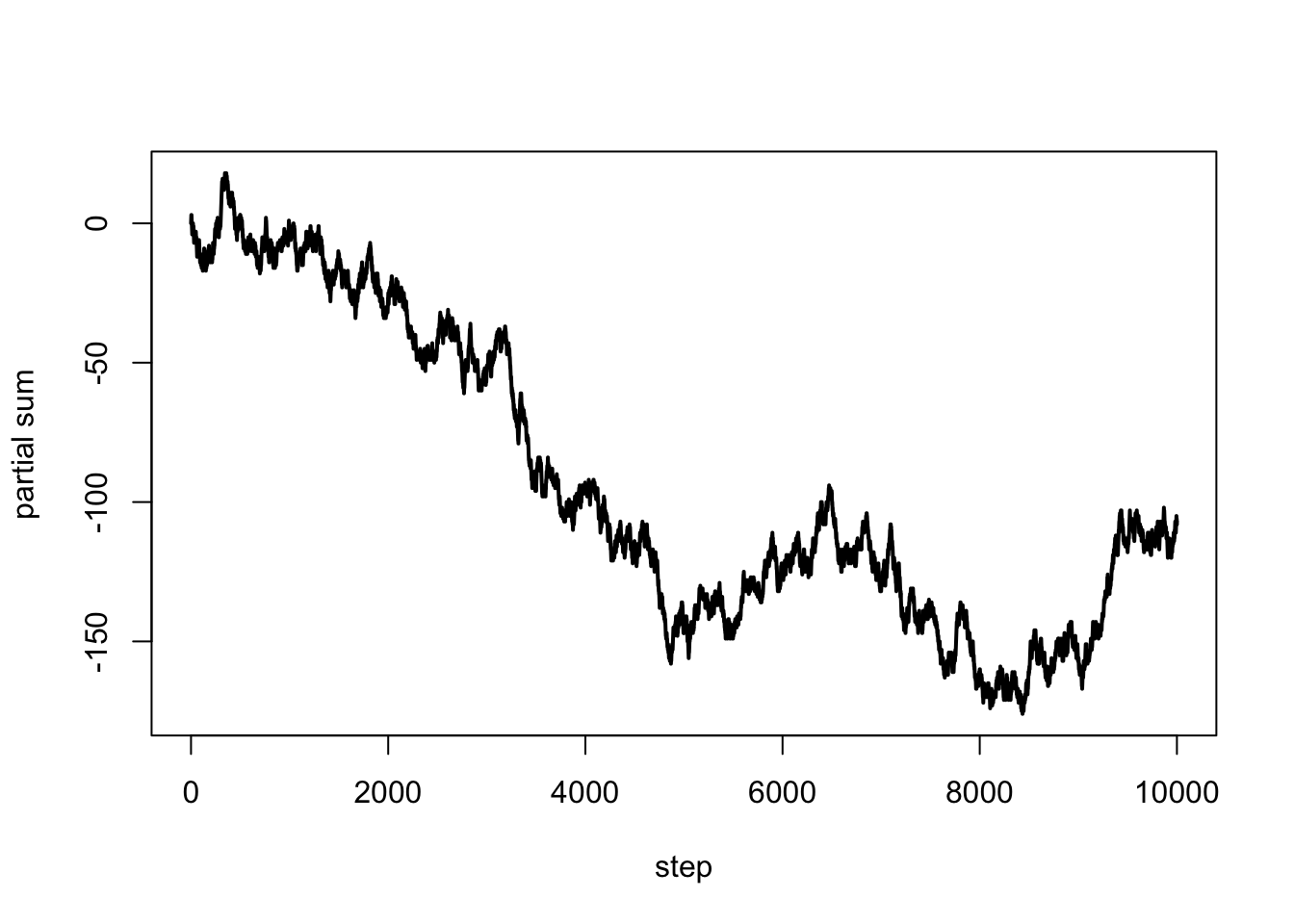
The following is an attempt to verify a result of Erdös and Rényi (closely related to the so-called Law of Iterated Logarithm). We plot the normalized partial sums, their cumulative maxima, and what the result predicts
t = s[-1]/sqrt(1:n) # normalized partial sums
plot(1:n, t, type = "l", lwd = 1, xlab = "step", ylab = "normalized partial sum", ylim = c(min(t), max(max(t), sqrt(2*log(log(n))))))
lines(1:n, cummax(t), lwd = 1, lty = 2)
lines(3:n, sqrt(2*log(log(3:n))), lty = 3)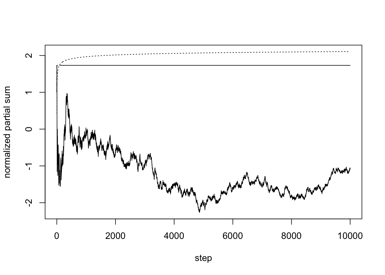
The convergence is very slow and not particularly obvious in this simulation. Most of the time, the maximum happens near the beginning of the normalized partial sum sequence (and this can be proved to be the case).
9.3 Galton–Watson processes
We work with a Poisson offspring distribution, as this is one of the most commonly studied example. The simple code below produces a realization of the sequence of population sizes over successive generations. It does not produce a fully detailed realization (which would have a tree structure).
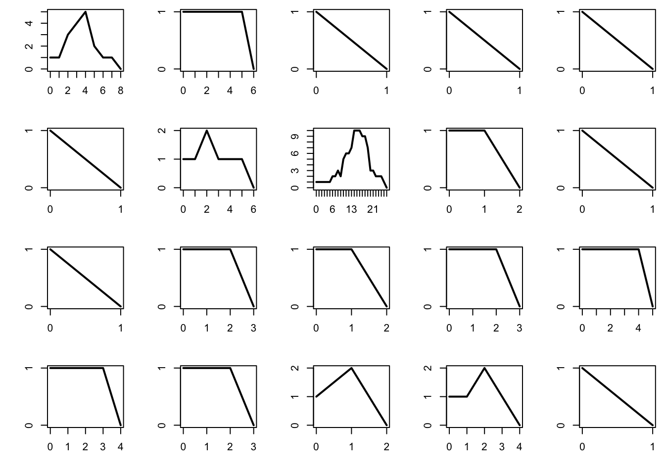
The probability of extinction is 1 if the mean number of offsprings per individual is \(\mu \le 1\), and is strictly positive if \(\mu > 1\). Below we plot the total population per generation for 20 different realizations of the process, and plot them. For computational reasons, we abort the process once the population reaches 1000 individuals, as this is a good indication that the process survives forever after that.
The subcritical regime corresponds to \(\mu < 1\). In that case, the process tends to die very quickly.
par(mfrow = c(4, 5), mai = c(0.5, 0.5, 0.1, 0.1))
mu = 0.9
n = 100 # maximum number of generations
for (b in 1:20){
  x = rep(0, n+1)
  x[1] = 1
  for (i in 1:n){
    x[i+1] = sum(rpois(x[i], mu))
    if (x[i+1] == 0) break
    if (x[i+1] > 1e3) break
  }
plot(0:i, x[1:(i+1)], type = "l", lwd = 2, xlab = "", ylab = "", axes = FALSE)
box()
axis(1, at = 0:i)
axis(2, at = 0:max(x))
} 
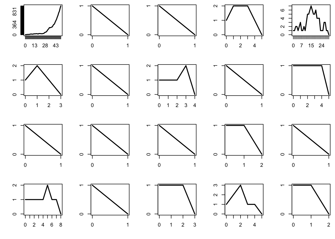
The critical regime corresponds to \(\mu = 1\). In that case the process dies eventually, but on occasion it will survive a relatively long time.
par(mfrow = c(4, 5), mai = c(0.5, 0.5, 0.1, 0.1))
mu = 1
n = 100
for (b in 1:20){
  x = rep(0, n+1)
  x[1] = 1
  for (i in 1:n){
    x[i+1] = sum(rpois(x[i], mu))
    if (x[i+1] == 0) break
    if (x[i+1] > 1e3) break
  }
  plot(0:i, x[1:(i+1)], type = "l", lwd = 2, xlab = "", ylab = "", axes = FALSE)
  box()
  axis(1, at = 0:i)
  axis(2, at = 0:max(x))
} 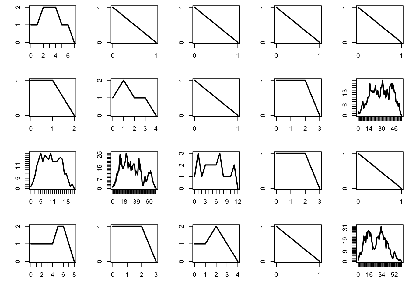
The supercritical regime corresponds to \(\mu > 1\). In that case, the probability that the process survives indefinitely is strictly positive. In addition, it turns out that, when the population survives, it increases exponentially in size — and this can cause trouble when performing simulations.
par(mfrow = c(4, 5), mai = c(0.5, 0.5, 0.1, 0.1))
mu = 1.1
n = 100
for (b in 1:20){
  x = rep(0, n+1)
  x[1] = 1
  for (i in 1:n){
    x[i+1] = sum(rpois(x[i], mu))
    if (x[i+1] == 0) break
    if (x[i+1] > 1e3) break
  }
  plot(0:i, x[1:(i+1)], type = "l", lwd = 2, xlab = "", ylab = "", axes = FALSE)
  box()
  axis(1, at = 0:i)
  axis(2, at = 0:max(x))
}