Chapter 24
The Dimension of the Solution Set of a Set of Polynomial Equations

Given a system of noncommuting polynomials S, one may wish to have some sense of how large the solution set is, i.e. the degrees of freedom. There are a number of possible approaches (none of which is perfect) to answering this question, and we outline one of them here. This method is useful and interesting of its own right, and is perhaps more valuable as an example in which the Groebner Basis algorithm can be used by pure algebraists.

24.1 The Commuting Case

If the polynomials S are members of a commutative affine polynomial (finite number of variables) ring, then there is a very classical way of computing the dimension of the solution set. One uses the Krull dimension or trancendance degree which are the same for affine commutative algebras. Daniel Lichtblau at Mathematica has written code that will do this.

24.2 Noncommutative Case: Gelfand-Kirillov dimension

Let R = k < x₁,...,x_n >, the polynomial ring over k in n noncommuting variables. The standard filtration on R is the sequence of vector subspaces of R, R_t, consisting of all polynomials of degree t or less. If I is an ideal of R, set T = R∕I. Then the standard filtration T_t on T is the sequence {R_t∕(I ∩ R_t)}. If we define H_T (t) = dim _k(T_t), the Hilbert series of T corresponding to this filtration is

The following dimension has been around since the 1960s and has become a main tool in noncommutative algebra. It was first introduced by I.M. Gelfand and A.A. Kirillov in a paper in 1966 describing work on enveloping algebras of Lie algebras. References for background and proofs of theorems are at the end of this chapter.

Definition 24.1 The Gelfand-Kirillov dimension of T is defined to be

We need a little bit more notation. Let A be an affine k-algebra, that is, an algebra finitely generated over a field k. Then A = k[V ] where V = Span_k{1,x₁,…,x_m} for some {x_j}⊂ A. Define

A quick fact about GK dimension: It is known that there exist algebras of GK dimension r for any real number r {0}∪{1}∪ [2,∞), and moreover no other number is attained.

There are several reasons that the Gelfand-Kirillov (hereafter abreviated GK) dimension is an apropriate measure of degrees of freedom. The following four standard theorems tell us that the GK dimension behaves much like the transcendance degree from commutative algebra. They follow easily from the definition, and a little combinitorics. Proofs can be found in the references at the end of the chapter.

Theorem 24.2 If A is a commutative algebra, then

Theorem 24.3 If B ⊂ A is a subalgebra, then

Theorem 24.4 If C is a homomorphic image of A, then

The following theorem shows that the GK dimension is well-behaved with respect to quotient algebras.

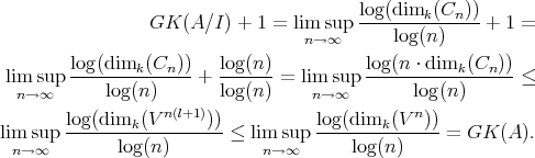
Theorem 24.6 Let A be an affine algebra and I an ideal of A that contains a left (or right) non-zero-divisor, c A. Then

Proof. Using the notation above, suppose c is a degree l non-zero-divisor. Let C_n be the vector space complement of
V ⁿ ∩ I in V ⁿ, So C _n ≃ V ⁿ∕(V ⁿ ∩ I). Note that the sequence {V ⁿ∕(V ⁿ ∩ I)} _n=1^∞ gives a filtration of A∕I. Now C_n ∩〈c〉 = {0}, as C_n ∩I = {0}. So C_n ⊕C_nc⊕⊕C_ncⁿ ⊂ V ^n(l+1) and the ⊕ are valid as acⁱ = bc^j,i < j implies cⁱ(a - bc^j-i) = 0 and c a left non-zero-divisor then gives a - bc^j-i = 0 so a 〈c〉∩ C _n which implies a = 0. So Thus

The computation of the GK dimension is in general difficult. Since the sequence whose limit is the GK dimension converges very slowly, the only hope is to compute some of the coefficients of the Hilbert series and then guess a generating formula for them. Then the GK dimension can be computed by taking the limit of this sequence. This may sound a bit ad hoc, but it has been implemented for several interesting algebras, an example of which follows.

The algebra we consider is the algebra on two variables generated by the relations that say that any two degree 2 monomials commute with each other. The commands used here are explained in the section on Commands.

We use the input file as follows:

The call to NCMakeGB finishes after only 2 iterations, so we know that the coefficients are being computed using a full Groebner basis, hence they are exact. The output is the following:

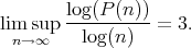
After staring at this sequence for a while, one sees that every other term is a square and the intermediate terms are products of sucessive integers after the 6th term. A formula then is [n][n + 1] where [a] is the greatest integer less than or equal to a. This is then clearly asymtotic to a quadratic polynomial. This sequence came from a gradation, so to get the sequence coming from the filtration we simply take the partial sums. This in turn will be asymtotic to a cubic polynomial in n, which we will call P(n). So the GK dimension of the quotient of the free polynomial algebra on two variables by the ideal generated by rels is:

24.3 References

1. Nastasescu, Constantin; van Oystaeyen, Freddy. Dimesions of Ring Theory.
2. McConnell, J.C.; Robson, J.C. Noncommutative Noetherian rings.
3. Krause, G.R.; Lenagan, T.H. Growth of algebras and Gelfand-Kirillov dimension.

24.4 Commands

The commands and algorithms were done by Eric Rowell with help from Dell Kronewitter and Bill Helton.

24.4.1 NCHilbertCoefficient[integer1, aListOfExpressions, integer2, anOption]

Aliases: none

Description: NCHilbertCoefficient[integer1,aListOfExpressions,integer2, anOption] attempts to compute the first integer1 coefficients of the Hilbert series for the algebra generated by the relations in aListOfExpressions. There are four possible calls to this function, here expressed in order of longest time used to least.

• The default (no fifth arguement) is for algebras that are nonhomogeneous. This will compute a (possibly partial) Groebner Basis out to integer2 iterations of Mora’s algorithm with respect to the ambient order, convert this basis to rules, and procede to compute the specified number of Hilbert series coefficients. Unless the partial Groebner basis computed contains all the polynomials that will ever appear in the (possibly infinite) full Groebner basis up to degree integer1, the dimensions of T_t computed will only be upper bounds.
• ExpressionForm → Homogeneous. This is only valid for homogeneous ideals. This does as above, only the resulting dimensions are for the standard gradation, and takes much less time. In theory, there should be no problem with the dimensions being inaccurate provided enough iterations are used. There is an algorithm for homogeneous problems that will return all the polynomials of a specified degree and less.
• ExpressionForm → partialGBHomogeneous. This is an option that will avoid the Groebner basis computation and simply convert the relations in aListOfExpressions to rules and use them to compute the Hilbert coefficients. This is useful particularly when one has already gone to the trouble of computing a (partial) Groebner basis. This is only coded for homogeneous ideals. The iteration number integer2 is ignored (although it must be there) so one may as well set it to 0.
• ExpressionForm → HomogeneousBinomial. This is a very specific option for ideals whose generators are the difference of two monic monomials (i.e. of the form: xyxz - yxzx). This is essentially the same as the homogeneous version above, only faster.

Arguments: integer1, aListOfExpressions, integer2, anOption

Comments / Limitations: The order is alway the ambient order. Make certain that your order is only length lexicographic as this will save time. There is no reason to use any order other than length lexicographic for Hilbert series computations that the author of this code can think of. Currently the with the default version of this function the ambient order will be cleared during the computation, as there is a new variable introduced that is later removed. For now, just remember to reset the order before proceding.

24.4.2 NCX1VectorDimension[alist]

Aliases: none

Description: NCX1VectorDimension computes the dimension of the span of a set of polynomials as a vector space over the ground field.

Arguments: alist

Comments / Limitations: none