The tools in the SYSTEMS package are designed to assist in studying various systems using the following commonplace idea (see [BHW] for more detail):
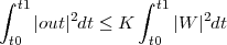
Define a finite-gain dissipative system to be a system for which
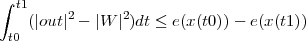
Define a storage or energy function on the state space to be a nonnegative function e satisfying
We find it convenient to say that a system of the above form is e-dissipative provided that the energy Hamiltonian H defined by
![T T T T
H = out out - W W + (p F[x,W ]+ F [x, W ] p )∕2](NCBIGDOC126x.png)
Theorem 44.1 (see [W],[HM]) Let e be a given differentiable function. Then a system is e-dissipative if and only if e is a storage function for the system. In this case, the system is dissipative.
Using this background, we may study dissipativeness of systems by examining the non-positiveness of Hamiltonians. Replacing the dual variables p by

![sHW = outT out - W T W + (∇x e F[x,W ]+ F [x,W ]T ∇Tx e)∕2](NCBIGDOC128x.png)
Often one finds that
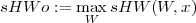
ruCritW=Crit[H,W]; (Calculate critical value for H w.r.t. W)
HWo=Sub[H,ruCritW]; (Substitute critical W back in H) sHWo=Sub[HWo,ruxz]; (Convert to state-space coordinates) |
since p is independent of W. Some examples are given later to illustrate.
What we have done so far is explain the very simplest case. Whenever one has a Hamiltonian which is quadratic in a variable our symbol manipulator optimizes the variable automatically. In H∞ control one gets Hamiltonians which are very complicated expressions in many variables (e.g. compensator parameters). One must take many maxima and minima in analysing these problems and we have found SYStems very effective at such computations.
Game theory is another area which produces Hamiltonians and calls for such computations.
Rather than try to list complicated classifications of Hamiltonian types that this addresses we proceed by presenting some examples. One is the classical bounded real lemma while the other derives the famous DGKF two Riccati equation formulas for nonlinear systems (which are affine linear in the input variables).
Also there is substantial systems capability in a completely different directions. NCAlgebra contains commands for manipulating block matricies. Since such computations are the substance of many results in systems theory it is already easy to do computations in these areas with NCAlgbra. A few formulas for 2 × 2 block matricies are stored: Schur complements, block LU decomposition, inverses, and Chain to scattering formalism conversions.