We think of this package as being useful for at least 4 things:
This package can be used with the NCAlgebra package to add powerful automatic methods for handling collections of equations in noncommuting variables.
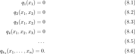
Most commutative algebra packages contain commands based on Gröbner Bases and uses of Gröbner Basis. For example, in Mathematica, the Solve command puts collections of equations in a “canonical” form which, for simple collections, readily yields a solution. Likewise, the Mathematica Eliminate command tries to convert a collection of polynomial equations (e.g., {pj(x1,…,xn) = 0 : 1 ≤ j ≤ k1}) in unknowns x1,x2,…xn to a “triangular” form in unknowns, that is, a new collection of equations like
The user who is not acquainted at all with Gröbner Basis should still be able to read and use most of the material which is contained within this document.
In [FMora], c.f. [TMora], F. Mora described a version of the Gröbner basis algorithm which applies to noncommutative free algebras. We refer to this algorithm as Mora’s algorithm and as the Gröbner Basis Algorithm. This strategy also puts collections of equations into a “canonical form” which we believe has considerable possibilities in the noncommutative case.
To learn how to install the program or use someone else’s installation, read Chapter ?? or Chapter ??.
The first thing you should do is read Part 1 to see examples of the basic commands.
If you are interested in simplification of expressions, you should read Chapter 9. Simplification is discussed in the papers [HW] and [HSW].
If you are interested in proving theorems and want to understand the ideas, you should read Chapter 16.
If you are interested in proving theorems and want to see examples, you should read Chapter 14. and Chapter 17 to see examples of the software in action.
If you want to understand the commands which were used to do the example in Chapter 14, then read Chapter 15.
If you want to compute Gröbner Bases, read Chapter 9.3 or read Chapter 20 without first reading anything else.
In addition,