15 Multiple Proportions
15.1 One-sample goodness-of-fit testing
We look at the Mega Millions lottery (https://www.megamillions.com/) which is in operation in most states in the U.S.. In the current version of the game, each draw consists of five balls sampled without replacement from an urn with white balls numbered \(1, \dots, 70\), and one ball (the “MegaBall”) sampled from an urn with gold-colored balls numbered \(1, \dots, 25\). Here are the draws for the year 2018
load("data/megamillions_2018.rda")
megaball = megamillions$Mega.Ball
megaball = factor(megaball, levels = 1:25) # just in case some numbers are absent
Although there is a case for direclty applying a test (to avoid the temptation of ‘snooping’), for illustration (and also because this is routinely done), we explore the data with summary statistics and plots
counts = table(megaball)
counts
megaball
1 2 3 4 5 6 7 8 9 10 11 12 13 14 15 16 17 18 19 20 21 22 23 24 25
6 4 3 4 4 3 3 2 7 5 6 5 5 5 1 4 5 3 3 6 3 5 8 2 2 colors = grey.colors(25, 0.1, 0.9)
barplot(counts, names.arg = 1:25, xlab = "Numbers", ylab = "Counts", main = "Bar chart", col = colors, las = 2)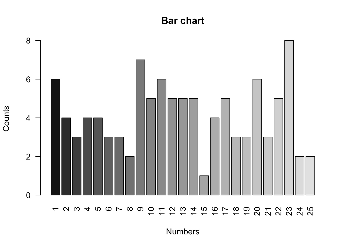
The main function that R provides for one-sample goodness-of-fit testing is the following, which computes the Pearson test, obtaining the p-value using the asymptotic null distribution (default) or Monte Carlo simulations. In the former case, the test statistic is “corrected” to make the approximation more accurate, and a warning is printed if the expected counts under the null are deemed too small for the approximation to be valid (as is the case with this dataset). If left unspecified, the null distribution is taken to be the uniform distribution on sets of values appearing at least once in the sample (hence the importance of making sure all possible values appear at least once, or are account for by specifying the levels as we did above).
chisq.test(counts)
    Chi-squared test for given probabilities

data:  counts
X-squared = 16.673, df = 24, p-value = 0.8623chisq.test(counts, simulate.p.value = TRUE, B = 1e4)
    Chi-squared test for given probabilities with simulated p-value (based
    on 10000 replicates)

data:  counts
X-squared = 16.673, df = NA, p-value = 0.8799
Even though the expected null counts are a bit small, the p-value based on an asymptotic approximation is quite accurate. The p-value being quite large (\(>0.30\)), there is no evidence against the null hypothesis — at least none provided by the test performed here.
15.2 Association studies
Consider the paper “Outcomes of Ethnic Minority Groups with Node-Positive, Non-Metastatic Breast Cancer in Two Tertiary Referral Centers in Sydney, Australia” published in PLOS ONE in 2014 (https://doi.org/10.1371/journal.pone.0095852). The primary purpose of this (retrospective) study was to examine in what respect Asian patients differed from Western patients referred to two tertiary cancer centers in South Western Sydney. We look at the age distribution
tab = matrix(c(154, 293, 79, 46), 2, 2)
rownames(tab) = c("<50", ">50")
colnames(tab) = c("Western", "Asian")
tab
Western Asian
<50 154 79
>50 293 46This 2-by-2 contingency table can be visualized with a segmented bar plot
barplot(tab, legend.text = c("<50", ">50"))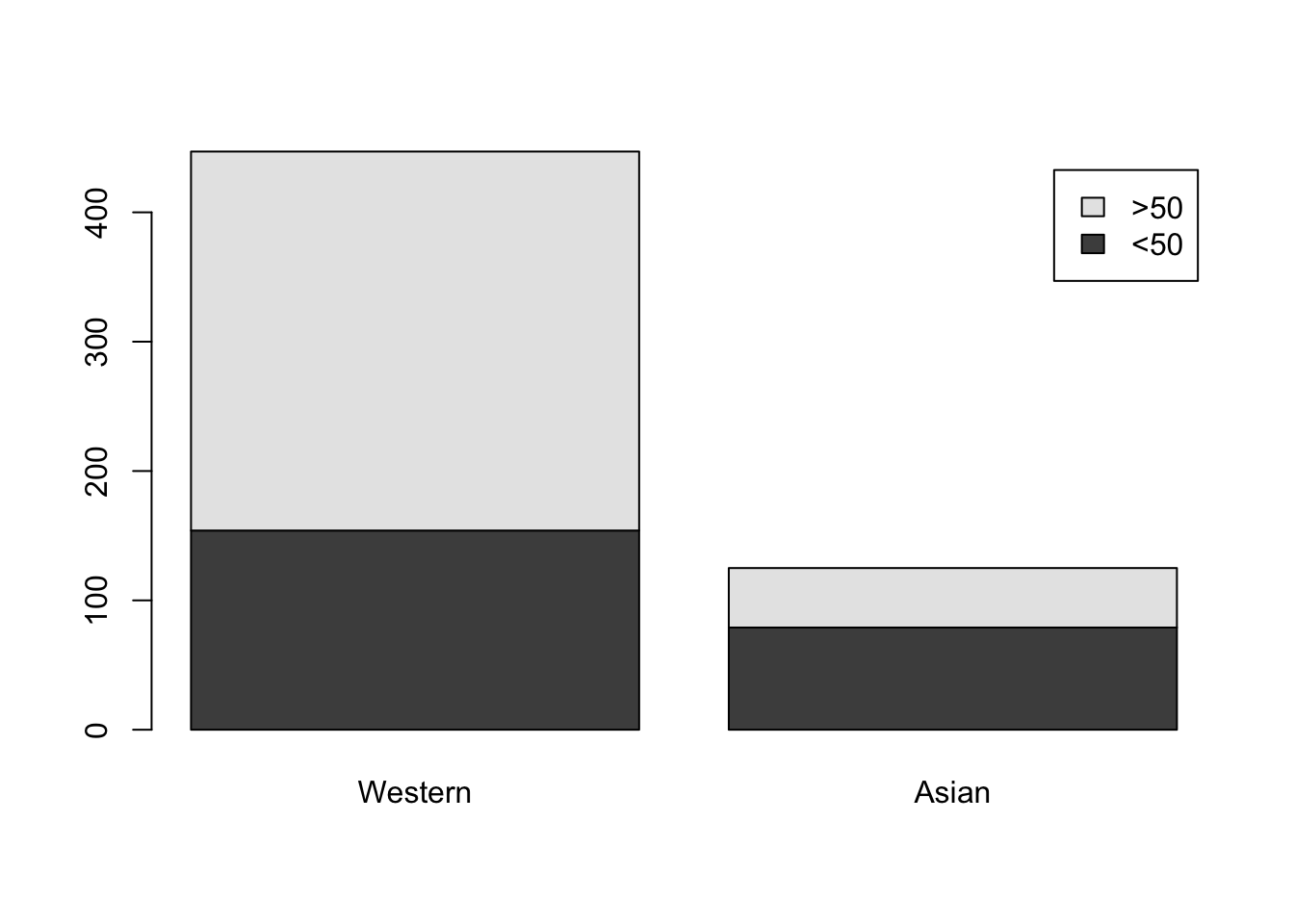
It’s pretty clear that Asian patients tend to be younger (at least based on the available age information), but let’s perform a test. In principle, this calls for a test of independence (aka a test of association). Such a test can be performed as follows, where the p-value is based on asymptotic theory with some correction improving the accuracy of the corresponding approximation
chisq.test(tab)
    Pearson's Chi-squared test with Yates' continuity correction

data:  tab
X-squared = 32.261, df = 1, p-value = 1.348e-08
Alternatively, conditioning on the margins (a form of conditional inference) leads to a permutation test
chisq.test(tab, simulate.p.value = TRUE, B = 1e4)
    Pearson's Chi-squared test with simulated p-value (based on 10000
    replicates)

data:  tab
X-squared = 33.441, df = NA, p-value = 9.999e-05
For a 2-by-2 contingency table, as in the present case, we can in fact compute the p-value exactly. This is the Fisher test. (The two p-values differ because the number of permutations above \(B = 10000\) is not large enough to properly estimate the actual permutation p-value.)
fisher.test(tab)
    Fisher's Exact Test for Count Data

data:  tab
p-value = 1.061e-08
alternative hypothesis: true odds ratio is not equal to 1
95 percent confidence interval:
 0.1978184 0.4713373
sample estimates:
odds ratio
 0.3067242
15.3 Matched-pair experiment
The following data comes from the paper “Evaluating diagnostic tests for bovine tuberculosis in the southern part of Germany: A latent class analysis” published in PLOS ONE in 2017 (https://doi.org/10.1371/journal.pone.0179847). The goal is to compare a new test for bovine tuberculosis, Bovigam, with the reliable but time-consuming single intra-dermal cervical tuberculin (SICT) test. For this, \(n = 175\) animals were tested with both, resulting in the following
tab = matrix(c(46, 119, 2, 8), 2, 2)
rownames(tab) = c("SICT[+]", "SICT[-]")
colnames(tab) = c("Bovigam[+]", "Bovigam[-]")
tab
Bovigam[+] Bovigam[-]
SICT[+] 46 2
SICT[-] 119 8It’s quite clear that the two tests, SICT and Bogigam, yield very different results, with Bovigam yielding many more positive results. This is confirmed by the McNemar test.
In its basic implementation, the p-value relies on the asymptotic null distribution with some correction to improve accuracy
mcnemar.test(tab)
    McNemar's Chi-squared test with continuity correction

data:  tab
McNemar's chi-squared = 111.21, df = 1, p-value < 2.2e-16
An exact version of the test is available from a package
require(exact2x2)
mcnemar.exact(tab)
    Exact McNemar test (with central confidence intervals)

data:  tab
b = 2, c = 119, p-value < 2.2e-16
alternative hypothesis: true odds ratio is not equal to 1
95 percent confidence interval:
 0.002012076 0.062059175
sample estimates:
odds ratio
0.01680672