18 Paired Numerical Samples
We work with a famous dataset consisting of the heights of men and their sons collected by Karl Pearson long time ago
load("data/father_son.rda")
attach(father_son)
18.1 Scatterplot
A scatterplot is an appropriate plot for paired numerical data. To deal with overlapping points, in the first plot we use small points, while in the second plot we use opacity. We add a diagonal line as it helps visualize the comparison.
plot(father, son, pch = 16, xlab = "father's height", ylab = "son's height", asp = 1, cex = 0.5)
abline(0, 1, lty = 2)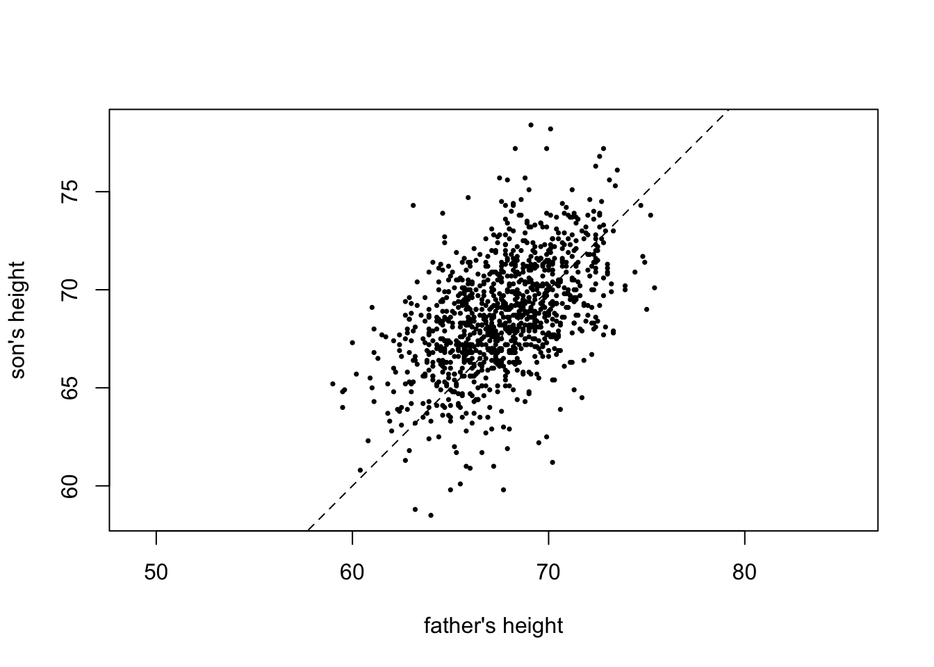
plot(father, son, pch = 16, xlab = "father's height", ylab = "son's height", asp = 1, col = grey(0, 0.5))
abline(0, 1, lty = 2, lwd = 2, col = grey(0, 0.5))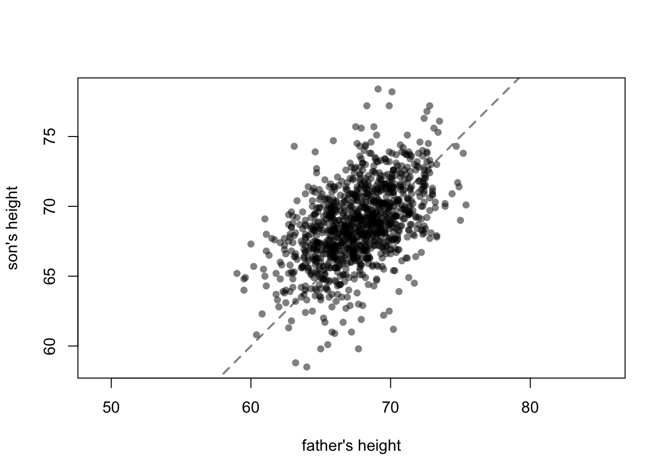
18.2 Testing for symmetry
The observations are paired (father, son). We take the difference and test for symmetry using the Wilcoxon signed-rank test.
wilcox.test(father, son, paired = TRUE)
    Wilcoxon signed rank test with continuity correction

data:  father and son
V = 168161, p-value < 2.2e-16
alternative hypothesis: true location shift is not equal to 0
There is overwhelming evidence that the distribution of the difference in heights is not symmetric (about 0). This is apparent when plotting a histogram, where we clearly see that a son tends to be taller than his father.
hist(son - father, breaks = 50, col = "grey", xlab = "difference in height (son - father)", main = "")
abline(v = 0, lty = 2, lwd = 2)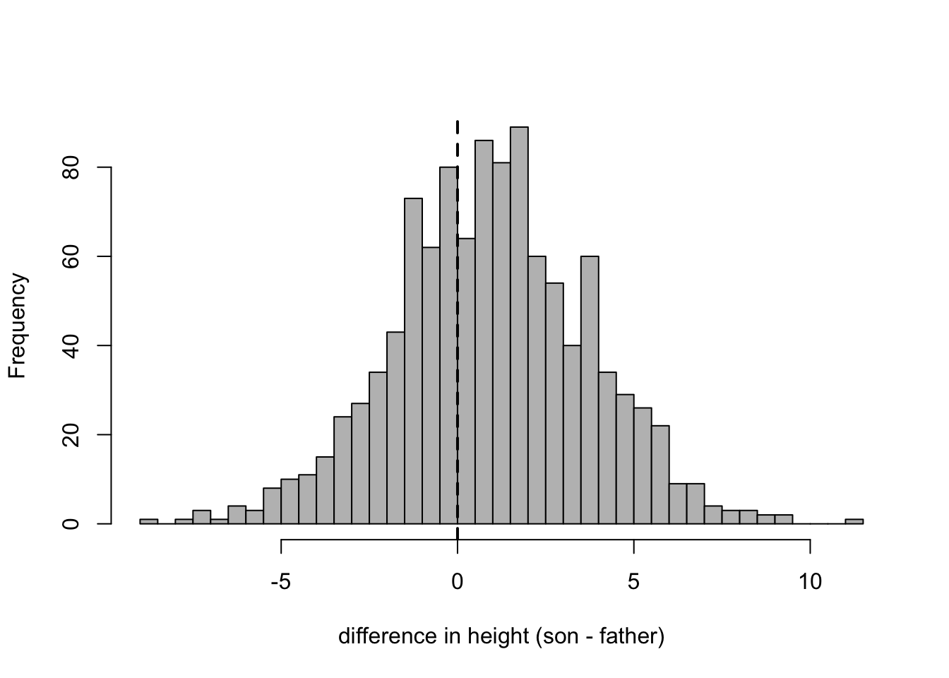
18.3 Repeated measures
We look at a data set on the effect of sleep deprivation on reaction time. 1In this longitudinal dataset, 18 subjects were followed over a 10 day period.
require(lme4)
days = 0:9
Data = sleepstudy[, -2] # removing Days
Data = unstack(Data)
matplot(days, Data, type = "b", pch = 15, ylab = "reaction time (ms)", col = grey(0, 0.5), lty = 1, lwd = 2)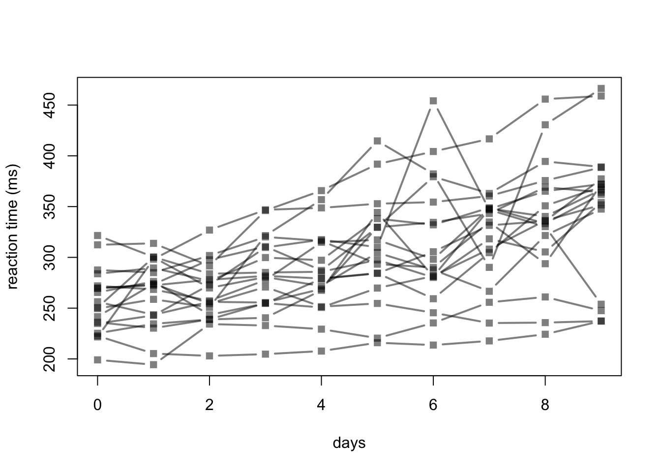
Although it’s clear that the reaction time increases with the number of days of sleep deprivation (as expected), for illustration, we apply the Friedman test. (Note that the subjects need to correspond to rows, so that we transpose the data. Also, the p-value relies on asymptotic theory.)
friedman.test(t(Data))
    Friedman rank sum test

data:  t(Data)
Friedman chi-squared = 86.085, df = 9, p-value = 9.904e-15