16 One Numerical Sample
The Extrasolar Planets Encyclopaedia (https://exoplanet.eu/) offers a catalog of confirmed exoplanets together with some characteristics of these planets. We focus on their mass.
load("data/exoplanet_mass.rda")
mass = sort(log(mass)) # we use a log scale
16.1 Quantiles and other summary statistics
summary(mass) # extremes, quartiles (including the median), and mean Min. 1st Qu. Median Mean 3rd Qu. Max.
-13.07357 -2.12026 -0.05129 -0.42477 1.13140 4.53903 range(mass) # the range giving the minimum and maximum[1] -13.07357 4.53903quantile(mass, c(0, 0.2, 0.4, 0.6, 0.8, 1)) # some sample quantiles 0% 20% 40% 60% 80% 100%
-13.0735732 -2.8949824 -0.4942963 0.4187103 1.5347144 4.5390304 median(mass) # sample median[1] -0.05129329mean(mass) # sample mean[1] -0.4247663sd(mass) # sample standard deviation[1] 2.372008The boxplot is based on the extremes and the quartiles. (In this particular version, no points are labeled as outliers. Note that this is not the default behavior of this function.)
boxplot(mass, range = Inf, horizontal = TRUE, col = "grey", xlab = "mass (log scale)")
rug(mass, lwd = 2) # adds a mark at each data points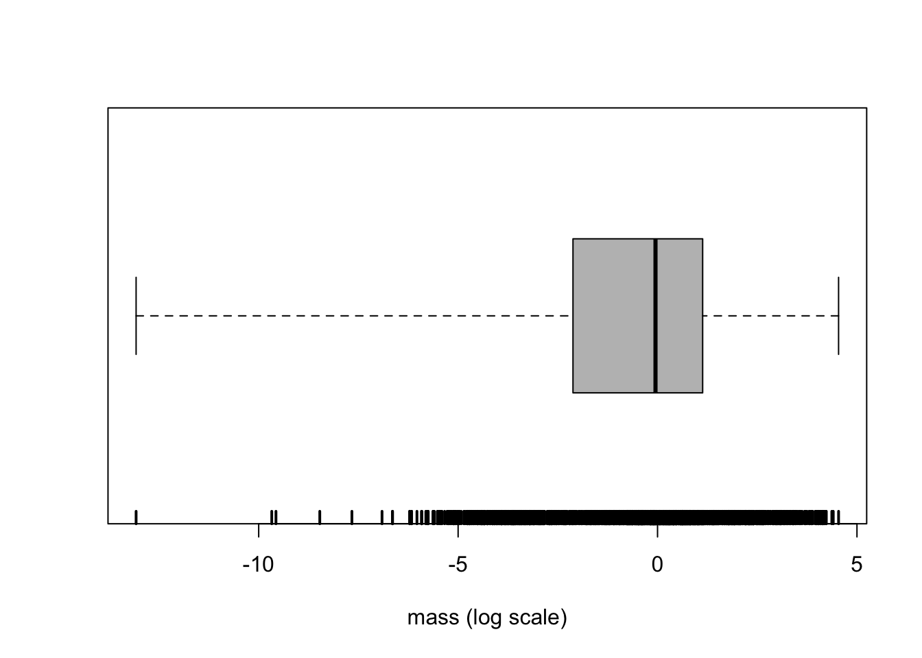
16.2 Empirical distribution function
Fun = ecdf(mass) # empirical distribution function
plot(Fun, lwd = 2, xlab = "mass (log scale)", ylab = "cumulative probability", main = "empirical distribution function")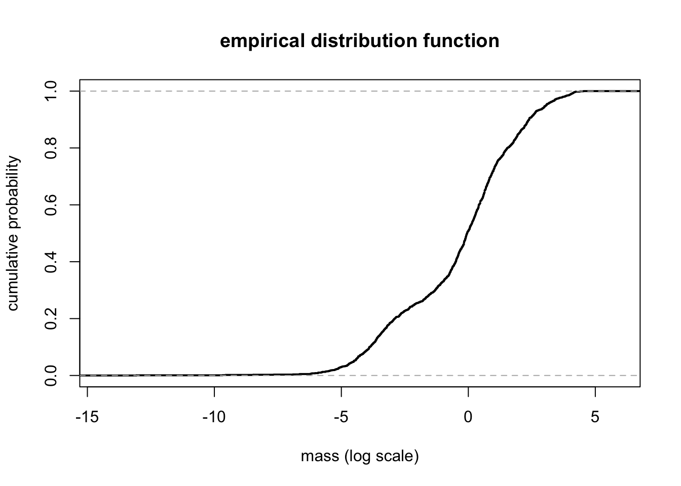
16.3 Histogram
hist(mass, col = "grey") # bins chosen automatically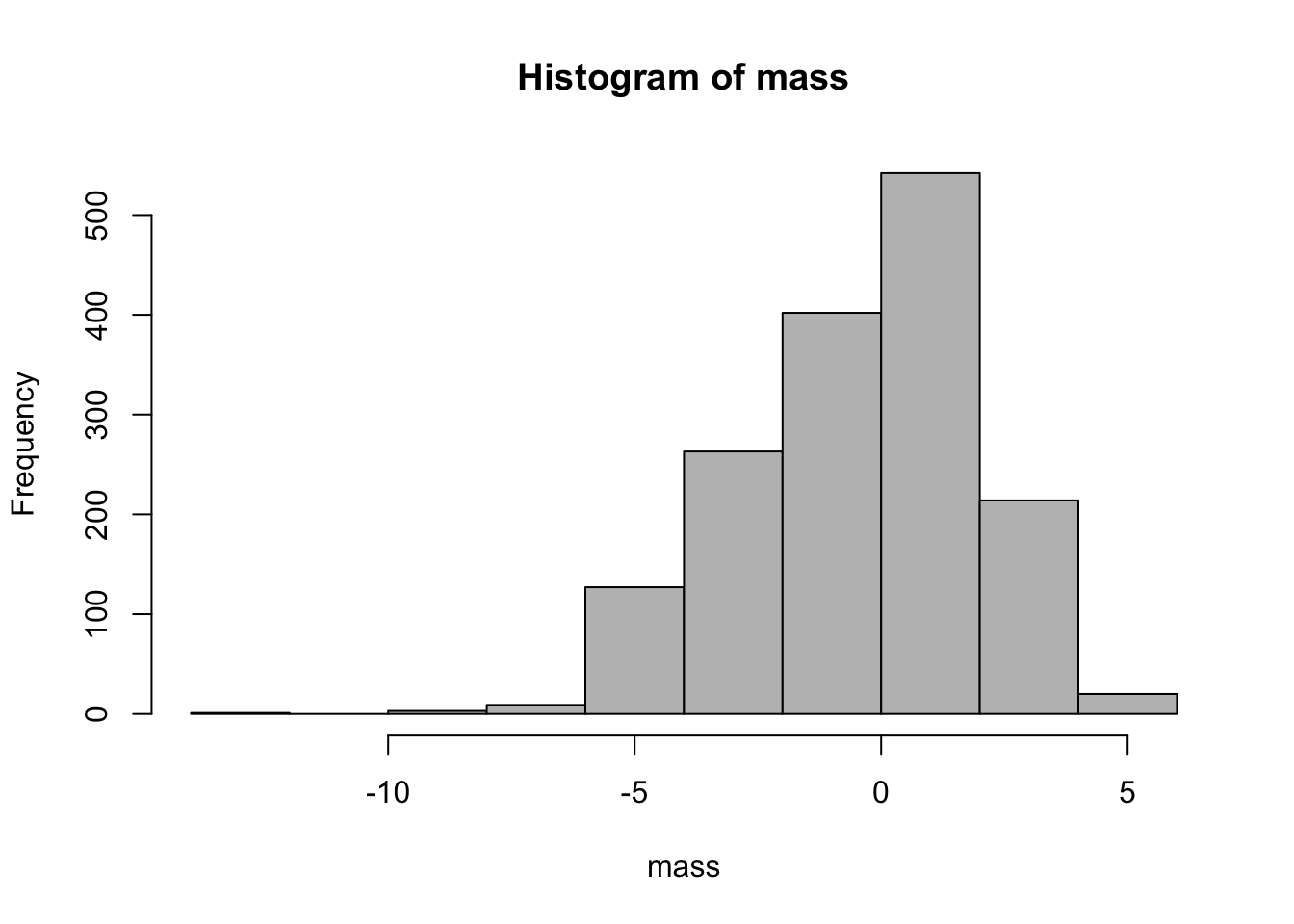
hist(mass, breaks = 100, xlab = "mass (log scale)", col = "grey") # set number of bins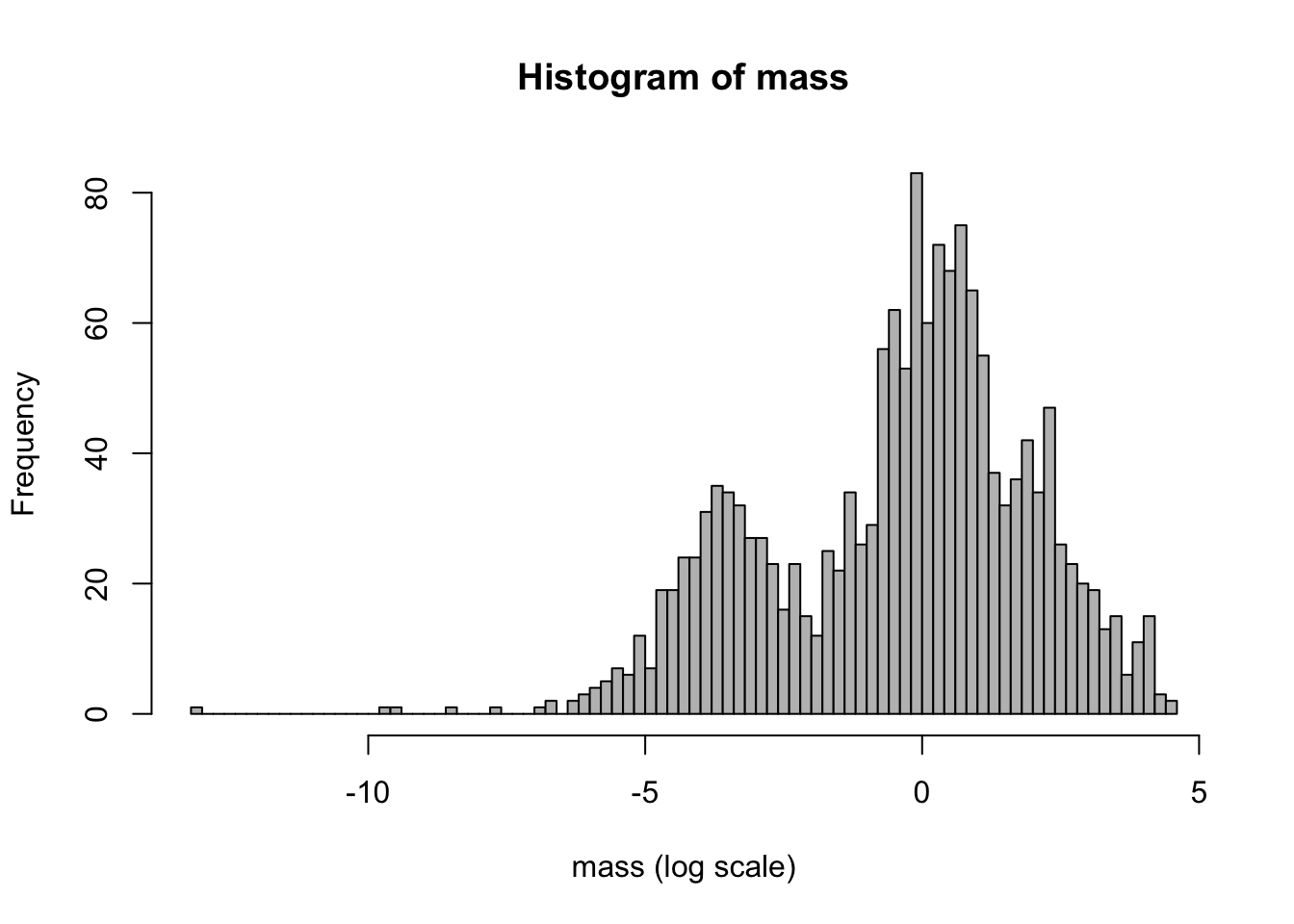
16.4 Confidence interval for the median
We compute a confidence interval for the median mass of an exoplanet in our system. There is an important caveat. It is not at all clear how the data we are using were collected, and chances are, it’s complicated given the context. In particular, it is not obvious that the sample we have available to us is in some real sense representative of the entire population of exoplanets ‘out there’. Nonetheless, in what follows, we pretend this is the case, and that in fact the sample is iid from that population. (Although arguably farfetched, this leap of faith is common in real data analysis.)
alpha = 0.01
n = length(mass)
q = 1 - pbinom(0:n, n, 1/2) + dbinom(0:n, n, 1/2) # refer to the book
tmp = which(q >= 1 - alpha/2)
lower = tmp[length(tmp)]
tmp = which(q <= alpha/2)
upper = tmp[1]
mass[c(lower, upper)] # 99% CI for the median mass (log scale)
[1] -0.1660546 0.1397619exp(mass[c(lower, upper)]) # 99% CI for the median mass (original scale)[1] 0.847 1.15016.5 Bootstrap confidence interval
With the same caveat, we move to compute a bootstrap confidence interval for the mean mass. We work in log scale. (If we want an interval in the original scale, we need to work in the original scale. This is because the mean, unlike the median, is not equivariant with respect to monotone transformations.)
Although it is straightforward to implement this by hand, for illustration purposes, we use a package. We compute the percentile bootstrap confidence interval. (Note that the level is approximate, as usual with bootstrap confidence intervals.)
require(bootstrap)
B = 1e4 # number of bootstrap replicates
mean_boot = bootstrap(mass, B, mean)
mean_boot = mean_boot[[1]] # bootstrapped means
int = 2*mean(mass) - quantile(mean_boot, c(1-alpha/2, alpha/2))
attributes(int) = NULL
int
[1] -0.5763911 -0.272772716.6 Kernel density estimation
We can visualize the sample density using a kernel density estimate. We superimpose it to a histogram. We explore the choice of different values for the bandwidth.
hist(mass, breaks = 100, freq = FALSE, col = "grey", xlab = "mass (log scale)", main = "")
# various choices of bandwidth
b = seq(0.1, 1, len = 10)
c = heat.colors(10, alpha = 0.5)
for (i in 1:10){
  lines(density(mass, bw = b[i]), lwd = 2, col = c[i])
}
lines(density(mass), lwd = 2) # default bandwidth
lines(density(mass, "ucv"), lwd = 2, col = "green") # CV bandwidth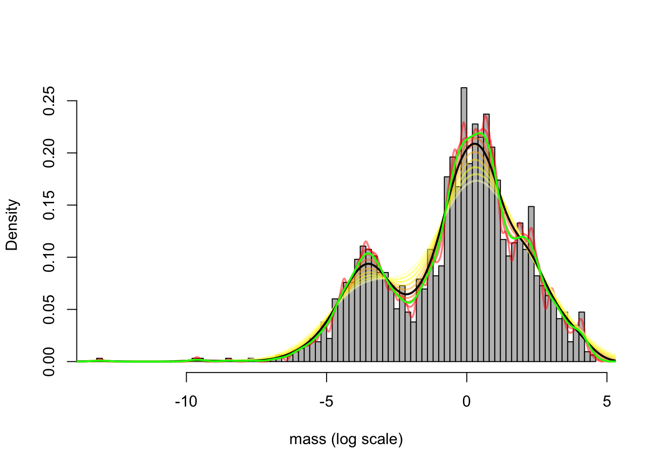
16.7 Kaplan–Meier estimator
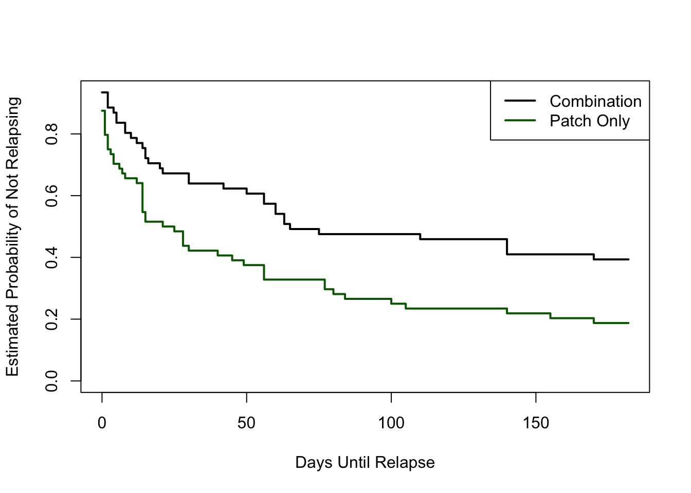
Censored data is commonplace in Survival Analysis. We a specialized package from that field. For illustration, we a dataset on smoking that is available in a different package, and with that dataset, we compute the Kaplan–Meier estimators for the two treatments groups. (Note that more variables are available in that dataset, but we only use time-to-relapse, relapse, and treatment group.)
require(survival)
require(asaur)
fit = survfit(Surv(ttr, relapse) ~ grp, data = pharmacoSmoking) # Kaplan--Meier curve
plot(fit, xlab = "Days Until Relapse", ylab = "Estimated Probability of Not Relapsing", lwd = 2, col = c("black", "darkgreen"))
legend("topright", c("Combination", "Patch Only"), col =  c("black", "darkgreen"), lty = 1, lwd = 2)